Rainbow array algebra #
Recent changes #
I’ve added a new section on the relation between bubbles and functional programming. I’ve also added a section about how simple neural networks like perceptrons can be expressed in rainbow terms. I’ve rewritten the transformers section for better clarity, accuracy, and completeness, including a description of multi-head attention and how we stack rounds of self-attention. Attention is paid throughout to how learned arrays appear.
Please feel free to ping me on Twitter for suggestions and feedback!
Introduction #
In the first post of this series, Classical array algebra, I set out a simple framework for thinking about how multidimensional arrays are manipulated in classical array programming. Please do read that first – there is terminology and notation that we’ll take for granted in this post.
In classical array algebra, we thought about arrays as functions – more precisely memorized functions aka lookup tables. Scalars were functions of 0 arguments, vectors were functions of 1 argument, matrices 2, etc. But think about a modern programming language like Python: while function arguments are normally distinguished by position f(1,2), we can also distinguish them by name f(x=1,y=2). This is a shift from seeing functions arguments as a tuple to seeing them as a dict.
In the world of arrays, this corresponds to a a new kind of array: one with named axes. But I’ll use color as a proxy for name, leading us to what I call rainbow array algebra. This simplifies and unifies many of the constructions we saw in the previous post, and to me, illustrates the possibility of a more humane kind of array programming.
Goals #
The goals of this post will be to:
-
briefly recap what we covered in the first post, including the idea of arrays-as-functions
-
understand this analogy is imposed a certain limited perspective
-
extend this perspective in a natural way, yielding rainbow arrays
-
re-examine the array operations from the first post in this new, colorful light
-
understand some traditional neural networks this way
-
explain the state-of-the-art Transformer architecture using rainbow circuits
-
provide some further reading materials
Recap #
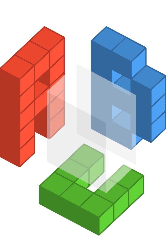
In the first post, we had in mind the following picture (and terminology) for an arbitrary array:
Of course, the number of axes can be arbitrary, and in applications like deep learning can easily be as high as 3 or 4. Note that role of color here is just as a visual aid! Axes are fundamentally identified by their position in the axes order associated with a given array.
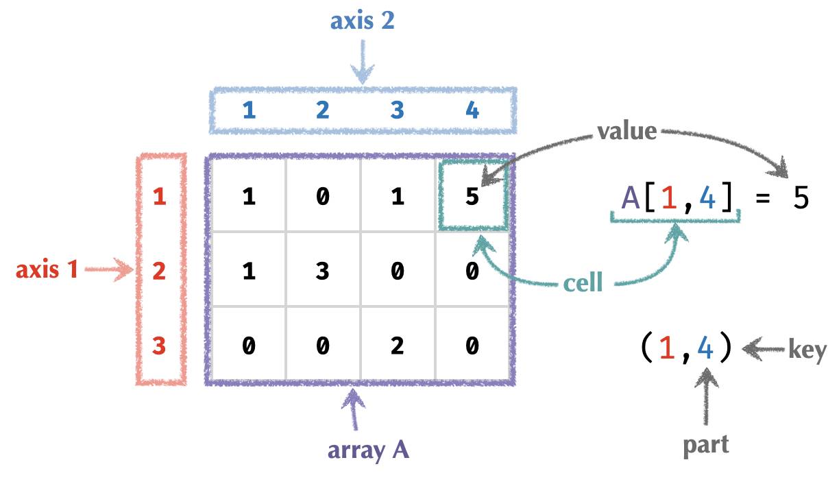
Given this picture, we identified n-arrays with functions of the form:
A : ⟨P1,P2,…,Pn⟩ -> V
The set ⟨P1,P2,…,Pn⟩ was called the key space, and V the value space.
We also thought of arrays as containers of elements from V, which are held within cells.
Each cell of an array is located by a tuple (p1,p2,…,pn) called a key, whose entries pi ∈ Pi are called parts, taking values from the associated part spaces Pi. The entire key is just an element of the key space. Parts and part spaces are sometimes called indices and index sets in array programming.
An axis i ∈ 1..n refers to the i‘th component of the key space.
A scalar is a 0-array with no axes. It has key space ⟨⟩ = { () }, and hence exactly one cell and value.
We presented an array using colorful half-frame notation, so a 3-array of shape ⟨2,3,4⟩ could be written:
⎡⎡[0 0 1 0 ⎡[0 1 1 1
⎢⎢[1 0 0 0 ⎢[0 0 1 0
⎣⎣[0 0 1 1 ⎣[0 1 1 1
We introduced a handful of operations that can be applied to either single arrays or combinations of them, listed here below:
| operation | meaning | cellwise definition |
|---|---|---|
| lift | apply f to matching cells |
f↑(A,B)[…] ≡ f(A[…], B[…]) |
| aggregate | use f to summarize axis |
fn(A)[…] ≡ f●∈■{ A[…,●,…] } |
| merge | collapse parts of an axis together | fRn(A)[…,●,…] ≡ f●∈■{ A[…,●,…] | R(●,●) } |
| broadcast | add constant axis | An➜[…,●,…] ≡ A[…] |
| transpose | permute (reorder) axes | Aσ[…] ≡ A[σ(…)] |
| nest | form array of arrays | An≻[…][●] ≡ A[…,●,…] |
| diagonal | fuse multiple axes together | A1:12[●,…] = A[●,●,…] |
| pick | choose cells by key | A[P][…] ≡ A[P[…]] |
Critique of classical array algebra #
Keys as tuples #
Classical arrays involve cells identified by keys, being tuples of parts. Tuples are simply ordered lists. Crucially, the fact that keys are ordered lists is what gives us an ordering for axes of an array, since axis n is just a “slice” through the n‘th component of the key space.
The natural question is: are tuples the best choice? What happens if we replace tuples with another data structure? What will this do to our notion of the axes of an array?
Certainly, tuples are simple, familiar data structures. In the functional perspective in which arrays are functions from key spaces to value spaces, tuples being keys correspond to the familiar idea of positional function arguments, which are currently the norm in software programming. This inspired the shorthand A[1,2,3] ≡ A( (1,2,3) ) for the cell of a 3-array.
Secondly, the commitment to ordered axes makes it easy to store the content of arrays. In a computer, the contents must be laid out in consecutive positions in linear memory (RAM). Ordered axes let us compute a memory location from key directly as long as we know the overall shape.
For example, the key (3,1,2) ∈ ⟨3,3,3⟩ yields an offset into linear memory:
offset = (3−1) * 9 + (1−1) * 3 + (2−1) = 19
Adopting this kind of addressing scheme is a requirement of executing array programs efficiently, since it permits us to avoid storing the keys themselves – every choice of key uniquely identifies a location in memory where the corresponding value can be found. Similarly, we can efficiently work backwards from a memory location to the corresponding key.
And so ordered axes have been woven into the fabric of classical array programming.
The problem with tuples #
As we have seen, composition of arrays require matching corresponding axes from the composed arrays. For example, tinging a color image with a tinting vector requires matching the tinting vector with the color axis of the image. So we would need two variants of a tinting function, one for the CYX image layout convention and one for the YXC convention, and make sure we call the right one!
In general, getting this matching right may require fiddly and error-prone transposition and broadcasting, with no surefire way to verify it at compile time. Worse, innocuous semantic changes can require cascading and non-local changes to an array codebase. For example, adding an additional axis to the input of an array program so that it operates on a vector of inputs to compute a vector of results can require rewriting many transpositions, broadcasts, and other operations.
Moreover, representing the axes of an array in this ordered way discards useful semantic information that might have been better kept around. This needless erasure of meaning is the source of countless bugs in array programming. The common solution is meticulous documentation of the source code of an array program to explain the interpretation of each axis at each point in a computation.
An analogy from historical computing #
This situation is eerily similar to one in the early days of computer programming. The registers that store temporary data in a CPU are numbered. Initially, code could only be written in the native machine code (or human-readable assembly code) of the CPU, and keeping track of what data was stored in which registers at which steps of a computation was a laborious exercise that taxed the memory and attention of the first human programmers.
Eventually, programmers invented higher-level programming languages which employed named variables, using automated compilers to translate the use and manipulation of these named variables into the corresponding manipulations of the CPU’s registers. Working with these names directly made programs much easier to read and write. In fact, these compilers often create more performant machine code, being able to analyze subtle tradeoffs that come from register use in different parts of the program.
A similar situation exists today with array programming, in which current array programming frameworks have forced array programmers into making choices about how axes should be ordered. Axis order can have a major impact on how array programs perform due to subtle effects such as cache locality. But rewriting your array program to exploit such opportunities is typically impractical. Just like in the early history of computing, we can anticipate a future in which array programmers can focus instead on what the axes mean and leave the optimal machine implementation and layout to tomorrow’s automated, autotuning compilers, which is exactly what we already do with register layout.
Further reading #
A far more thorough critique than I present here can be found at the excellent “Tensors considered harmful”.
Rainbow arrays #
Introduction #
As we eluded to, our main move is to replace the role of the tuple in our key spaces with a data structure called a record. These records will encode the same part information but will label the axes with explicit axis names, rather than having axes be implicitly labeled by their linear order in the tuple. But what exactly is a record?
Records #
Let’s take an example key tuple for a 3-array:
(5,3,2)
And replace it with a record, which is a structure we will write like this:
(a=5 b=3 c=2)
The tuple has components labeled by 1, 2, and 3. The record has fields labeled by a, b, and c.
Relationship to axes #
As we saw, the relationship tuples have to axes is that the n‘th axis is associated with the n‘th component of every key tuple.
With records, we instead have that the axis named a is associated with the a field of every key tuple.
Therefore, record keys are the natural counterpart to tuple keys when we name our axes instead of number them.
Relationship to shapes #
Before, we saw that a shape like ⟨3,2,4⟩ denotes a Cartesian product, which is the set of tuples:
⟨3,2,4⟩ ≡ { (i,j,k) | 1≤i≤3, 1≤j≤2, 1≤k≤4 }
Switching to records, we can create a record shape ⟨a=3 b=2 c=4⟩ that creates a set of records:
⟨a=3 b=2 c=4⟩ ≡ { (a=i b=j c=k) | 1≤i≤3, 1≤j≤2, 1≤k≤4 }
Rainbow notation #
However, instead of writing a record as (a=3 b=2 c=4), we color code the fields via a,b,c and write simply (3 2 4):
(3 2 4) ≡ (a=3 b=2 c=4)
Note that in this notation we have dropped commas, because the structure (3 2 4) is not a tuple (where order of components matters), but a rainbow notation for a record (which has no order of fields).
Similarly, the colored shape of a matrix with 3 rows and 4 columns under the color coding row,column is:
⟨3 4⟩ ≡ ⟨4 3⟩ ≡ ⟨row=3 column=4⟩
Notice order here is inconsequential, it is color that becomes the notational carrier of axis label information.
We can further adapt our array algebra notation to reflect this orderless, color-based semantics.
Array lookup #
For array lookup, we replace A[●,●,●] with A[●●●]. Notice again the lack of commas, since:
A[●●●] ≡ A[●●●] ≡ A[●●●] ≡ …
Similar to before, the cell value A[●●●] is still shorthand for function application on a record A( (●●●) ).
The full syntactic desugaring under the ambient color coding a,b,c looks like this:
A[●●●] ≡ A( (●●●) ) ≡ A( (a=● b=● c=●) )
Shape #
As before, we will indicate the colorful shape of an array by writing a “partial function signature” that describes its key space. Here, a matrix with 3 rows and 4 columns is written:
M : ⟨3 4⟩
When we don’t wish to state explicit values, we will as before use squares:
M : ⟨■■⟩
Axes #
We will denote the set of axes of an array A with axes(A) or A. An axis is just a color, of course, so to write down such an abstract color we will use a colored ◆ symbol:
S : ⟨⟩ -> V         axes(S) = S = {}
V : ⟨5⟩ -> V        axes(V) = V = {◆}
M : ⟨3 4⟩ -> V      axes(M) = M = {◆,◆}
A : ⟨2 2 2⟩ -> V    axes(A) = A = {◆,◆,◆}
Role of color #
To summarize the role of color in our notation systems with a table:
| name | example | role of order | role of color |
|---|---|---|---|
| classic notation | A[i,j,k] |
primary | none |
| colorful notation | A[i,j,k] |
primary | visual aid |
| colorful notation | A[●,●,●] |
primary | replace symbols |
| rainbow notation | A[ijk] |
visual aid | primary |
| rainbow notation | A[●●●] |
none | primary |
Notice that in both rainbow and colorful notation, we can but need not replace the role of symbols i,j,k with tokens ●,●,● to denote unique parts of a key tuple / record.
Examples redux #
Let’s re-examine the case of our color image, whose subpixels are shown here:
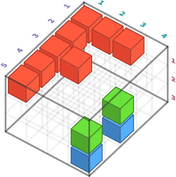
Below we’ve highlighted a particular green (c=2) subpixel at spatial position y=3 and x=4:
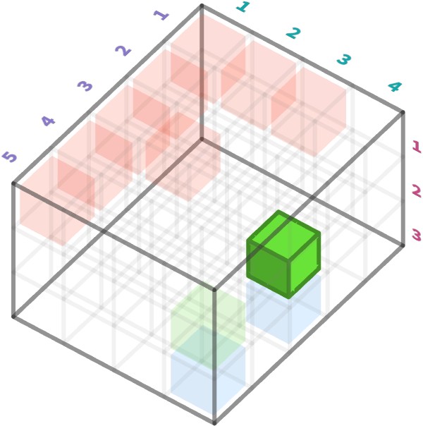
Here is the classical versus rainbow view of this cell, under coding YXC:
| paradigm | shape of array (keyspace) |
key of subpixel |
|---|---|---|
| classical | ⟨5,4,3⟩ |
(3,4,2) |
| record | ⟨y=5 x=4 c=3⟩ |
(y=3 x=4 c=2) |
| rainbow | ⟨5 4 3⟩ |
(3 4 2) |
Rainbow circuits #
In the last post, we saw examples of array circuits, which depict graphically how arrays can be composed with one another. Parts flow down from the input ports along purple wires. Similarly, array cell values flow down the page to output ports.
For example, a matrix defined by adding a vector to the rows of another matrix is defined cellwise like this:
A[r,c] ≡ M[r,c] + V[c]
This has the corresponding circuit:
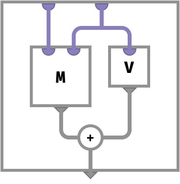
Here, the ports that take key parts are ordered from left to right. For rainbow arrays, we eschew order and of course color the ports instead. For example, let us take the following cellwise definition:
A[●●] ≡ M[●●] + V[●]
This corresponds to the following rainbow circuit:
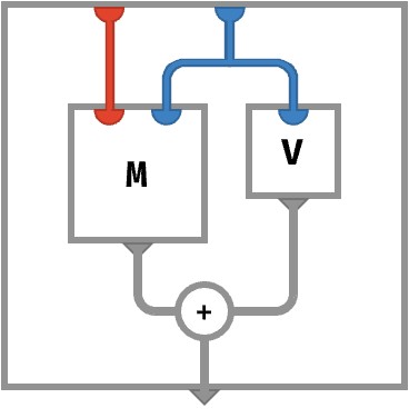
Unlike with classical array circuits, the order of ports and wires does not matter, only their color. In general, we can deduce the type of an array depicted in this way by reading the colors of the ports present on the top edge of its frame. The outermost frame is the array or function we are defining with a circuit, the inner frames are intermediary arrays that we are computing, or for labeled boxes, arrays whose values we are using in the definition.
Reorganizing the API #
How do rainbow arrays reformulate our algebra? Here’s a quick summary:
| operation | change in rainbow world |
|---|---|
| lift | automatically broadcast over missing colours |
| aggregate, merge, nest |
parameterized by color rather than order |
| transpose | meaningless; axes are not ordered |
| broadcast | redundant |
| pick | unchanged |
| recolor | new operation – equivalent of transpose |
In short, we mostly eliminate one operation from our API – broadcasting – since it becomes largely redundant owing to the increased flexibility of map operations over their lifted cousins.
Perhaps more importantly, we gain clarity about the intended semantics of our operations, since the axes preserve their “semantic role” across compositions.
Let’s examine in detail how the operations of classical array programming change now that we are under the rainbow.
Rainbow operations #
Aggregate, merge, nest ops #
For rainbow arrays, the earlier operations of aggregation, merging, and nesting remain largely as before. The only difference is that they are parameterized by axis color rather than by axis number.
For classical arrays, we wrote an axis-parameterized operation as, for example:
sum2(A)
(or sum2 in colourful notation). But if our axes are not ordered, and color is the only distinction between axes, we use a coloured symbol ◆ that identifies the relevant axis:
sum◆(A)
The color-generic representation of this particular aggregation operation is:
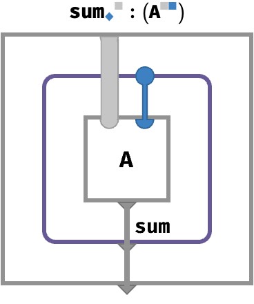
The purple frame is something we saw in the first post: it is syntax sugar for multiset subcircuit. In brief, for any given setting ● of the gray wire bundle, the subcircuit collects the cell values A[●●] corresponding to all possible settings for ●, and then sums them. In other words, given ●, it computes sum● { A[●●] }.
Axis genericity #
But there is a new convention here as well: the thick light-gray wire stands in for an arbitrary bundle of non-blue wires – the way the circuit works is independent of which of these extra wires are present (if any). This is a core benefit of rainbow arrays: when we parameterize operations by color, they become totally generic with respect to other axes that may or may not be present in the arrays they operate on. In contrast, classical array algebra is context sensitive. For example, an aggregation over axis 2 has a meaning that depends on what other axes are present: if we prepend a new axis to the input array, the meaning of this aggregation will change in a way that doesn’t reflect our original intent.
Lift / map op #
We saw that for classical arrays, lift and broadcasting operations are often combined to perform common operations like matrix multiplication.
For rainbow arrays, the broadcasting step is naturally subsumed under the lift step. The mechanism arises from the fact that all arrays that participate in an lift operation must have the same colourful shape. If any of the arrays have shapes that have fewer colours than necessary, there is a unique way they can be broadcasted to have the right colors (= named axes). The resulting array will then have the union of the colors of all the inputs. This means there is a unique array operation for each operation of the underlying value space, as long as the arrays being combined have “compatible shapes”.
We will name this new, more flexible operation map.
Let’s look at some examples to make things clearer.
Vector times vector #
We’ll start by multiplying two vectors. Because each vector has a single axis and therefore a single color, there are two possibilities: the colors match, or they don’t.
First, let’s consider matching colors; for example, the multiplication of two ■-vectors. The shapes of the inputs and output of the mapped * are:
     U : ⟨■⟩
     V : ⟨■⟩
U *↑ V : ⟨■⟩
The cellwise definition can only be one thing, corresponding to the familiar lift multiplication of two classical vectors:
(U *↑ V)[●] ≡ U[●] * V[●]

[1 2 3 * [0 1 2 = [0 2 6
Next, let’s consider non-matching colors, the multiplication of a ■-vector and a ■-vector:
     U : ⟨■⟩
     V : ⟨■⟩
U *↑ V : ⟨■■⟩
According to our rule, we broadcast U to have a blue axis and V to have a red axis to make their shapes compatible, which implies a unique cellwise definition:
(U *↑ V)[●●] = U➜[●●] * V➜[●●]
             =  U[● ] *  V[ ●]
Here, we introduce the notational shorthand A➜ to mean that an array is broadcast to have a colored axis with suitable part space. Hence, our cellwise definition of *↑ on these shapes is determined uniquely to be:
(U *↑ V)[●●] = U[●] * V[●]
Let’s see a concrete example:
          ⎡0    ⎡[0 0 0    ⎡[0 1 2
[1 2 3  * ⎢1  = ⎢[1 2 3  = ⎢[0 2 4
          ⎣2    ⎣[2 4 6    ⎣[0 3 6
Note the special feature of rainbow arrays that we can lay out their axes in any order we choose, as long as the brackets are colored correctly! This is a reflection of the fact that there is no canonical order of axes, only their canonical color. For classical arrays, the opposite was true: only the order of nested brackets mattered, their color was merely a visual aid to communicate how axes between several arrays corresponded.
Array times scalar #
A scalar array S has no colors, and so there is no possibility of sharing. Here we illustrate this for a vector:
     S : ⟨⟩
     V : ⟨■⟩
S *↑ V : ⟨■⟩

(S *↑ V)[●] ≡ S[] * V[●]

2 *↑ [1 2 3] = [2 4 6]
And for a matrix:
     S : ⟨⟩
     M : ⟨■■⟩
S *↑ M : ⟨■■⟩

(S *↑ M)[●] ≡ S[] * M[●●]

2 *↑ ⎡[1 2 3 = ⎡[2 4 6
     ⎣[3 2 1   ⎣[6 4 2
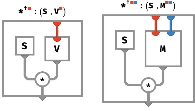
The rainbow circuit for this kind of situation is depicted below, for scalar-times-vector on the left and scalar-times-matrix on the right:
Matrix times matrix #
For two matrices, there are 3 possibilities for sharing:
| z | z | z |
|---|---|---|
M : ⟨■■⟩ |
N : ⟨■■⟩ |
2 shared colors |
M : ⟨■■⟩ |
N : ⟨■■⟩ |
1 shared colors |
M : ⟨■■⟩ |
N : ⟨■■⟩ |
0 shared colors |
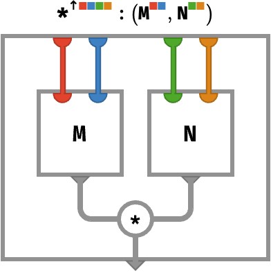
Let’s start with full sharing, where we are multiplying two ■■-matrices:
     M : ⟨■■⟩
     N : ⟨■■⟩
M *↑ N : ⟨■■⟩

(M *↑ N)[●●] ≡ M[●●] * N[●●]

⎡[1 2 *↑ ⎡[0 1 = ⎡[0 2
⎣[3 4    ⎣[1 0   ⎣[3 0
This is the classical lift-multiplication. The rainbow circuit for this kind of situation is depicted below:
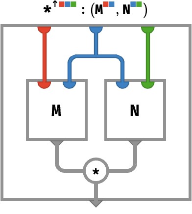
Next we have one shared color, where we are multiplying ■■-matrix and a ■■-matrix:
     M : ⟨■■⟩
     N : ⟨■■⟩
M *↑ N : ⟨■■■⟩

(M *↑ N)[●●●] ≡ M[●●] * N[●●]

⎡[1 2 *↑ ⎡⎡0 ⎡1 = ⎡⎡ 1*⎡0  2*⎡1  = ⎡⎡⎡0 ⎡2
⎣[3 4    ⎣⎣1 ⎣0   ⎢⎣   ⎣1    ⎣0    ⎢⎣⎣1 ⎣0
                  ⎢⎡ 3*⎡0  4*⎡1    ⎢⎡⎡0 ⎡4
                  ⎣⎣   ⎣1    ⎣0    ⎣⎣⎣3 ⎣0
The rainbow circuit for this kind of situation is depicted below:
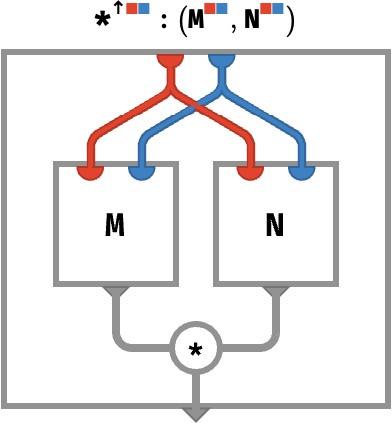
Finally, we have the case of zero shared colors, where we are multiplying a ■■-matrix and a ■■-matrix:
     M : ⟨■■⟩
     N : ⟨■■⟩
M *↑ N : ⟨■■■■⟩

(M *↑ N)[●●●●] ≡ M[●●] * N[●●]

⎡[1 2 *↑ ⎡[0 1 = ⎡⎡⎡[0 1 ⎡[0 2
⎣[3 4    ⎣[1 0   ⎢⎣⎣[1 0 ⎣[2 0
                 ⎢⎡⎡[0 3 ⎡[0 4
                 ⎣⎣⎣[3 0 ⎣[4 0
This is a kind of “matrix nesting”, where each cell of one matrix is replaced by a scaled copy of the other matrix, with that scaling factor being the corresponding value from in the cell of the first matrix. It doesn’t matter which matrix we choose to nest inside the other – as long as our choice matches the order of axis nesting when we write the result down.
The rainbow circuit for this kind of situation is depicted below:
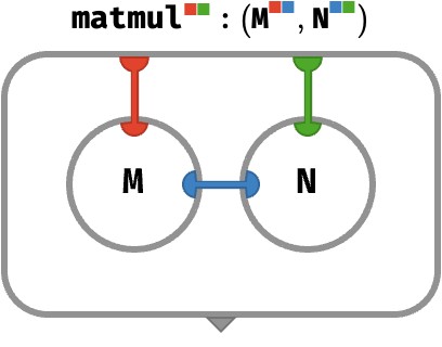
Matrix multiplication #
We are now in a position to construct matrix multiplication by mapping * over matrices that share a single color, and then aggregating that color:
    M : ⟨■■⟩
    N : ⟨■■⟩
M ⋅ N : ⟨■■⟩

(M ⋅ N)[●●] ≡ sum●∈■{ M[●●] * N[●●] }

M ⋅ N ≡ sumM⋂N (M *↑ N)
Here recall that A refers to the set of colors of A, so that M ⋂ N gives the set of shared colors:
M ⋂ N = {◆,◆} ⋂ {◆,◆} = {◆}
As a rainbow circuit, this looks like:
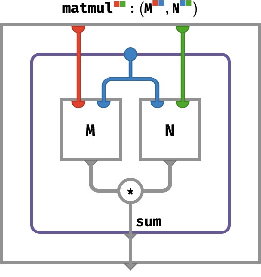
We will abbreviate this kind of situation by introducing some graphical sugar in the form of tensor networks, which are bubbles that do not explicitly route array values, and instead assume that any “internal wires” that do not have an explicit port on the bubble participate in a multiset sum as above. Using this convention, matrix multiplication above can be depicted as:
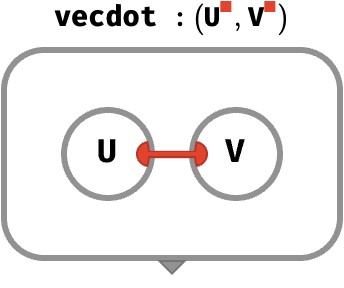
Inner product #
The above definition of rainbow dot product gives us exactly the correct definition of the inner product between two same-colored vectors U and V:
    U : ⟨■⟩
    V : ⟨■⟩
U ⋅ V : ⟨⟩

U ⋅ V ≡ sumU⋂V(U *↑ V)
      = sum◆  (U *↑ V)

(U ⋅ V)[] = sum●∈■{ U[●] * V[●] }
          = U[1] * V[1] + U[2] * V[2] + …
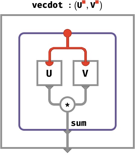
The tensor network depiction of this is:
General rainbow dot product #
The general form of this rainbow dot product A ⋅ B applies to pairs of arrays A,B and produces an array that has the symmetric difference △ of the colors of A and B, meaning the colors that are in one shape but not in both:
    A : J -> V
    B : K -> V
A ⋅ B : (J △ K) -> V

A ⋅ B ≡ sumA⋂B (A *↑ B)
Here, we are adopting the convention that set operations like J △ K applied to shapes occurs fieldwise, so that:
⟨5 3⟩ ⋃ ⟨3 6⟩ = ⟨5 3 6⟩
⟨5 3⟩ ⋂ ⟨3 6⟩ = ⟨3⟩
⟨5 3⟩ △ ⟨3 6⟩ = ⟨5 6⟩
⟨5 3⟩ - ⟨3 6⟩ = ⟨5⟩
As a more complex example, let’s consider the general rainbow dot product V ⋅ A between a vector V:⟨■⟩ and a 3-array A:⟨■■■⟩:
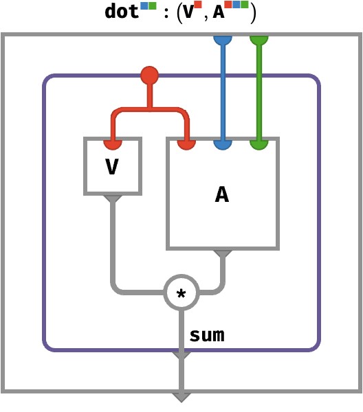
As a tensor network, this looks like:
What is the “general picture” of rainbow dot product between two arrays A and B? We cannot use actual colors in a rainbow circuit, since we wish to depict a situation that applies when A and B have arbitrary colors. What we can do instead is use thick wires that stand in for sets of wires with varying colors, with the understanding that all such sets are disjoint. We will still color these thick wires, but these colors serve an indexing role, referring to entire sets of individually colored wires. Using this convention, the arbitrary rainbow dot product is:
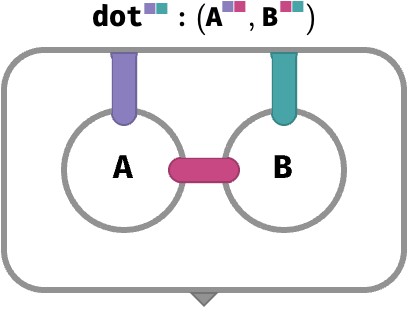
Even though it represents an infinite family of diagrams (depending on what color wires are present on A and B), this diagram is uniquely defined for any A and B! This is because the only way these wire bundles can be “color-disjoint” and still add up to the available colors of A and B is if the wires between A and B have colors A ⋂ B, the wires between A and the outer frame have colors A \ B, and those between B and the outer frame have colors B \ A.
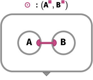
Contraction #
A more explicit building block that we will use in coming sections is broadly known as contraction. Under the rainbow, this will take the form of colored contraction, where we choose a single shared axis of two arrays, multiply the two arrays along that axis, and sum that axis away. We’ll denote this with ⊙:
The simplest case is when both arrays are vectors that have only this axis. This produces a scalar:
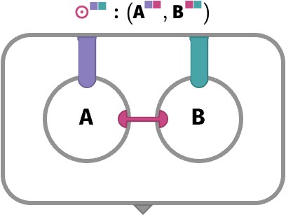
But in general, they can have any additional axes, which will be preserved. This is just the general semantics of rainbow mapping, which extends any operation on arrays to include arbitrary additional axes that aren’t otherwise part of its definition:
Example: tinting an image #
As a practical example of how rainbow mapping can streamline array programming, let’s look at a particularly simple example: tinting a color image.
Recall that a color image can be represented as an classical array of shape I:⟨H,W,3⟩ (here using the YXC convention).
Let’s say that we wish to change the color balance of this image, by doubling the intensity of the blue channel, and keeping the other channels the same. This tinting factor can be represented as a 3-vector:
T : ⟨3⟩ = [1 1 2]
The operation tint(I, T) of tinting I by tinting factor T can be defined cellwise as:
tint(I, T)[y,x,c] ≡ I[y,x,c] * T[c]
In terms of our classical array API, this can be achieved by broadcasting T over the first (Y) and second (X) axes followed by an lift-multiplication with I:
tint(I, T) = I *↑ T1➜H,2➜W
In practice, array programming library recognize this form of broadcasting and do not actually actualize the array T1➜,2➜ in memory. The resulting computation is closer in spirit to our cellwise definition above.
In the rainbow world, we have two important changes: firstly, the image has colorful shape I:⟨H W 3⟩, which does not involve any choice of axis convention, and so any definition of tint has no need to pick a convention.
Secondly, we can achieve the tinting operation simply as mapping I * T:
tint(I, T) ≡ I *↑ T

(I * T)[y,x,c] ≡ I[y,x,c] * T[c]
This is not merely a benefit in simplicity. It also means that the exact same definition of the tint operation will work on an array representing a video, in which an additional time axis T is present that represents a sequence of successive image frames:
V : ⟨T H W 3⟩

tint(V, T)[t,y,x,c] ≡ V[t,y,x,c] * T[c]
General cellwise definition #
Having seen a variety of examples of mapping, we can take a stab at a formal definition of map f.
To do this, we will introduce a slight notational convenience, which is to write the array type K->V more compactly as VK (this is a kind of “stepped down” version of the way we write the set of functions from A to B as BA).
 f : (V  , V  , … , V  ) -> V

A1 :  VK1
A2 :       VK2
 ⋮
An :                VKn

f↑ : (VK1, VK2, … , VKn) -> VK
 K =   K1 ⋃ K2 ⋃ … ⋃ Kn
The situation is depicted below in a rainbow circuit for n=3:
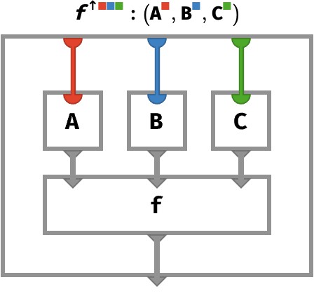
Even this is not quite general enough, since the function f could take arguments of varying type, and issue yet a third type. We will now switch to coloring rather than numerically indexing the arguments, so that f takes arguments of types V,V,…,V and returns a type V, and the arrays A,A,…,A are of type VK=K->V:
 f : ( V,  V, … ,  V) ->  V

 A :  VK
 A :      VK
 ⋮
 A :              VK

f↑ : (VK, VK, … , VK) -> VK
 K =   K ⋃ K ⋃ … ⋃ K
The use of color in this example is quite different from the use of color elsewhere in this post – we are simply using it as an alternative to numbered indexing of the arguments of f and the arrays Ai. But it certainly suggests that we could consider functions that operate on records rather than tuples. In that case, the use of color would accord with that of rainbow notation, where color identifies the field of a record.
Let us explore this generalization with a rainbow circuit:
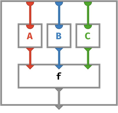
The only change here is that the input wires of the mapped function f are also colored, indicating the function takes a record with fields red, blue, and green. We will leave this intriguing possibility for a future section.
Recolor op #
We just stated the transposition is made redundant by moving to rainbow arrows. For classical arrays, transposition reordered axes but preserved arity; recoloring is similar.
As a canonical example, let’s consider the colored version of the familiar operation of transposing a matrix, which interchanges the roles of rows and columns.
Initially, let’s work without any of our syntax sugar, relying on explicit record notation. However, we will still use the ambient color coding a,b,c to make things easier to follow.
Say we have a matrix M:⟨a=2 b=3⟩ but we want a matrix M̂:⟨a=2 c=3⟩. Essentially, we want to rename the axis b to have name c.
However, as is typical of cellwise definitions, we must work backwards, since we must translate cell lookups of the array we want, M̂, to cell lookups of the array we have, M.
Conceptually, we must apply a function 𝜎={a↦a,c↦b} to the fields of the key for M̂ to obtain keys for M. We will write this with the same superscript notation as classical transpose:
Mc↦b[(a=i c=j)] ≡ M[(a=i b=j)]
In the superscript we’ve skipped the field a, which isn’t renamed. But it’s clear that what 𝜎 is operating on keys as follows:
𝜎( (a=i c=j) ) = (a=i b=j)
Now let’s mix in the syntactic sweetener, which we avoided because it makes things look almost too trivial!
Our recoloring operation will turn a matrix M:⟨■■⟩ into a matrix M◆↦◆:⟨■■⟩. It is defined cellwise as:
M◆↦◆[i j] ≡ M[i j]
In other words, the action of 𝜎 = {◆↦◆} on keys is:
𝜎((i j)) = (i j)
Note that in the discussion above we are using the symbol ◆ to indicate purely an axis color, not a particular size (■) or part (●).
Lambdas and closures #
In the first post, we touched on the topic of nesting and unnesting. In the simplest (rainbow) case, nesting turns a matrix M into a vector-of-vectors V = M≻, unnesting turns a vector-of-vectors V into a matrix M = V≺:
M  :       ⟨■■⟩ -> V
M≻ : ⟨■⟩ -> ⟨■⟩ -> V

V  : ⟨■⟩ -> ⟨■⟩ -> V
V≺ :       ⟨■■⟩ -> V
Through the lens that arrays are functions, nesting corresponds to currying, and un-nesting to uncurrying. But it doesn’t stop there.
When we drew the array circuit for nesting, we introduced bubble notation, which enclosed a circuit with a thick gray border to indicate that it was used as a value. Such a value could be piped around with thick gray wires, and returned as the contents of a cell in another array. Let’s show the rainbow circuit for M≻, which is the circuit that produces the “row vectors” of M (if we consider M to have rows and columns).
Let’s explain what this really means! In functional programming terms, what we are doing here is in fact very interesting: we are using the functional programming features of lambda functions and closures. I’ll explain.
First, notice that the entire array we are defining has one red input port and one array-valued output port. Hence, it is ■-vector, whose cells are themselves arrays.
Let’s consider what happens when this nest operation is evaluated, meaning we have specified a particular part value ● at the top red port and are trying to obtain an output value on the bottom triangular port. The value of this output port is the following bubble that appears in the interior:
This bubble show above represents an array with one blue input port, thus it is a ■-vector. Functionally, this bubble represents a lambda function, an anonymous function / array that we are creating during the computation of the larger circuit. Clearly, this anonymous function contains the entire matrix M as internal data. It also captures a piece of the environment, specifically the part ● flowing along the red wire at the time the bubble was created.
When this anonymous function is later used (outside the circuit), it will be provided a value ● for its blue input wire, and it will return the value of the corresponding cell M[●●]. In other words, once we have evaluated the circuit for M≻ (“asking for a particular row vector”), we get a ■-vector that contains that row, which we can then ask for any particular column of that row.
In functional programming terms, we have first created and then evaluated a closure, one that has closed over the value ●.
Cellwise, we have the following definition:
M≻[●][●] ≡ M[●●]
Reading from left to right: we first lookup the cell ● of M≻, obtaining a closure, and then evaluate that closure at ● to obtain a scalar value M[●●].
In summary, the operation M≻ turns a ■■-matrix M into a ■-vector whose cells contain ■-vectors, and it does this by constructing closures over ●-values.
Efficiency #
Nesting and unnesting operations as defined by closures are not typically used in array programs, since vectors-of-vectors are not efficiently constructable in most array programming languages. Instead, such operations are implicit in the way matrices, etc. are used. To make these operations efficiently representable, more sophisticated type systems and compilers are needed. This is arguably a limitation of today’s popular array frameworks, which do not model array programming as higher-order functional programming, despite the conceptual elegance it offers.
Neural networks #
One of the places where the need for named axes / rainbow arrays is most acute is in the field of deep learning, owing to the intricacy of modern neural network architectures and the number of axes that are simultaneously involved. So, to exercise some of the formalisms we’ve built up, let’s start by expressing two classical kinds of feedforward neural network.
First, we’ll formulate the simplest kind of neural network, a perceptron, often used as a building block for larger networks.
As a second exercise, we’ll stack several perceptrons together to form a multilayer perceptron (MLP), a kind of network that illustrates the “deep” in deep learning.
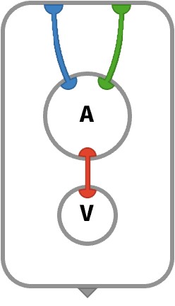
Perceptrons #
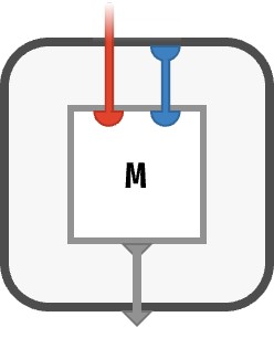
A perceptron, which we’ll abbreviate as an SLP (for single-layer perceptron), is the simplest possible example of an artificial neural network.
An SLP operates on an input vector I to produce an output vector O, using two learned parameters: a weight matrix W and a bias vector B. It is defined as follows:
    I        : ⟨■  ⟩
       W     : ⟨■ ■⟩
          B  : ⟨  ■⟩
SLP(I, W, B) : ⟨  ■⟩

SLP(I, W, B) ≡ (W ⊙ I) + B
In terms of linear algebra, W ⊙ I is the equivalent of ordinary matrix-vector product W ⋅ I. This is clearer with the cellwise definition:
SLP(I, W, B)[●] ≡ sum●(W[●●] * I[●]) + B[●]
Here is the corresponding circuit:
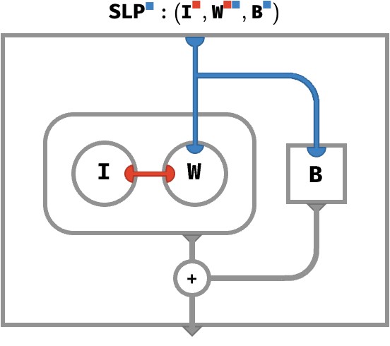
The interior tensor network bubble expresses the contraction W ⊙ I, and each component of the resulting vector is added to the corresponding component of the B vector.
Notice that this entire circuit is computing the output vector O: the outer frame has a single blue port, which confirms the circuit expresses a ■-vector.
Abstracting the input #
You might have noticed that something doesn’t feel quite right about this circuit.
What’s the problem? The ■-vector I, which is conceptually the “input” to this neural network, is living inside the circuit, along with the weights and biases. How can we instead feed the input I to the circuit, and get the output ■-vector O as result?
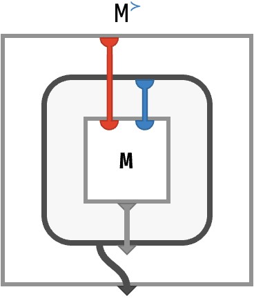
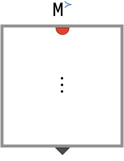
As we saw in the previous section, we can achieve this by putting the above circuit into a bubble:
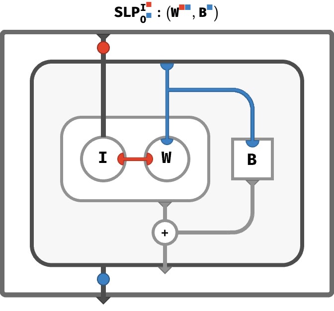
Here, we’ve used our previous circuit as a subcircuit: the dark gray bubble inside a new, larger circuit. This larger circuit defines a function to transform input vectors to output vectors. It accepts an array via the input port, pipes it along the thick, dark gray wire into the bubble, to the I node, where it is contracted with W matrix. Likewise, it pipes the entire output vector circuit (the dark gray bubble) to the output port of our operation. The little medallions on these dark wires are hints about the axes that are present on the array these wires carry.
Clearly, the arrays I, W, and B are playing two different roles in this circuit. Those two roles are captured in the type signature atop the diagram:
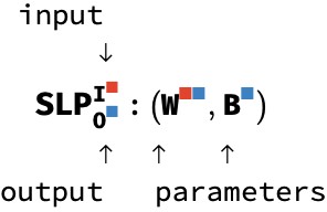
The signature records the input array I as a superscript and the output array O as a subscript, showing their respective shapes. In contrast, the weights and biases W and B remain as internal arrays to this circuit. We can think of the SLP operation as a higher-order function which constructs a circuit from parameters W and B, where this circuit consumes vector I and emits vector O.
If this is a bit mind-bending, don’t worry too much. This syntax just helps us distinguish internal parameters – arrays that are embedded in a circuit – from explicit input and output arrays that are carried on wires. It is the internal parameters that are trained by back-propagation, whereas the inputs and outputs are fed with training data.
Multilayer perceptrons #
A perceptron is a building block, and the simplest thing to build is a tower. This yields a multilayer perceptron, or MLP.
In an MLP, which consists of a tower of \(n\) MLPs, the output vector of each SLP has a non-linear function like ReLU applied to it (elementwise), and the result is used the input to the next SLP in the tower. Here’s the circuit diagram:
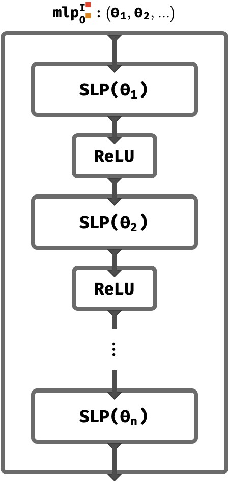
You can see that each SLP in the tower has independent weights and biases Wi and Bi, which we abbreviate here as just ϴi.
MLPs have much greater representative power than single perceptrons, owing both to the non-linearity and the ability to form complex internal representations that are built up step-by-step.
Transformers #
Now that we’ve seen how perceptrons work, a more thorough worked example of rainbow array thinking comes from understanding the basic mechanism of the Transformer architecture. Transformers are a family of deep neural network architectures that have shown astonishing promise in modelling human language via autoregression: predicting the next token in a sequence of tokens that represents written language. They form the basis of the wildly popular ChatGPT and related technologies.
This section will illustrate using rainbow circuits how transformers are built. We won’t discuss more complex topics like gradient descent, teacher forcing, or loss functions. The aim is to get a sense of how self-attention actually works – focusing specifically on the shapes of the arrays that are being manipulated. Rainbow arrays provide a key advantage, since they let us keep all the various axes in view at the same time, learning why they exist and what they mean.
Transformers vs. recurrent neural networks #
Like recurrent neural networks (RNNs), transformers operate on sequences. In an RNN, a sequence of input vectors is processed one at a time. Information flows in from each successive input vector, and is used to update a hidden state in a way that depends on the type of RNN (e.g. classical, LSTM, GRU). At a high level, the information flow in an RNN is like this:
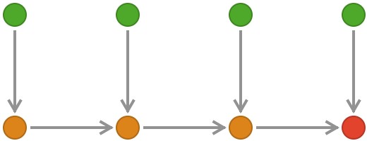
In a textual RNN, these input vectors are derived from tokens, e.g. the letters of a string. Each token yields one such “token vector”, and these are processed in a serial fashion, yielding at the end of a sequence a final hidden state that can be used for prediction (to predict the next token, in the case of generative / autoregressive networks) or classification (e.g. sentiment analysis). But RNNs can operate on other kinds of sequence, like financial and medical time-series or audio signals.
In contrast, transformers do not have this serial architecture. The entire sequence of token vectors is updated in parallel in a series of rounds of so-called self-attention. Each token vector is allowed to make queries against the other token vectors, and the results of these queries inform the update of that particular token vector. A technical detail: for generative transformers, the query from a token vector is only applied to tokens prior to it in the sequence – this is called causal masking.
At a high level, the information flow is like this, where we show 3 rounds before the final token vectors are obtained:
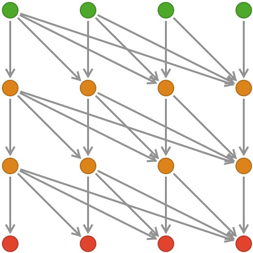
Let’s unpack all this!
Input encoding #
A transformer represents text as a sequence of tokens. For simplicity we can think of these tokens as being individual Unicode symbols that represent units of human writing (in current implementations the tokens are usually variable length “chunks” of Unicode symbols that are learned via a separate process). In computer science parlance, these sequences of Unicode symbols are called strings. A string of length N is a 1-array of type:
S : ⟨N⟩ -> U
where the value space U is the set of Unicode symbols: U = {a,b,c,d,…}. As an example, take the length 5 string abcba, which corresponds to the 5-vector:
S = [a b c b a
The first step is to turn the string into a sequence of token vectors that can be operated on by the transformer. These token vectors have some size T.
We do this by encoding this string vector into a matrix, where each symbol is “embedded” as an T-vector of real numbers via a dictionary D that defines which symbol u ∈ U should go to which vector ⟨T⟩ -> ℝ:
D : ⟨U⟩ -> ⟨T⟩ -> ℝ
If we use the toy alphabet U = {a,b,c}, we might define a corresponding dictionary D that uses one-hot vectors to represent these symbols as 3-vectors:
      a  b  c
    ⎡⎡1 ⎡0 ⎡0
D = ⎢⎢0 ⎢1 ⎢0
    ⎣⎣0 ⎣0 ⎣1
Our example string vector abcba encodes to the ⟨53⟩ matrix:
    ⎡⎡1 ⎡0 ⎡0 ⎡0 ⎡1
V = ⎢⎢0 ⎢1 ⎢0 ⎢1 ⎢0
    ⎣⎣0 ⎣0 ⎣1 ⎣0 ⎣0
The general recipe is: a length N input string S encodes into an ⟨NT⟩-matrix by using each character to pick the corresponding T-vector from D, and unnesting these vectors into a matrix:
V : ⟨N T⟩ -> ℝ
V = D[S]≺
So far, this seems simple, and is in fact how strings are encoded for prior architectures. We elide an interesting detail here, which is about positional encoding, a process by which additional information about where each token’s position in the string is injected into the corresponding token vectors.
Attention #
Overview #
We are now ready to describe the process of iterated self-attention that forms the basis of the transformer architecture. It is founded on an attention step, which takes a query, a sequence of keys, and a sequence of values, and produces a result which is weighted sum of those values. Each weight in the sum is derived from the relevance of that key to the query – we’ll describe how shortly.
This is a kind of weighted database lookup – the result of a query is not a single value in a database but a weighted sum of all values, with values considered more relevant to the query being weighted more highly than values that are less relevant. This kind of weighting of all possible results is typical of deep neural networks, because it allows backpropagation to measure the contribution of every possible element of the sequence, and shift attention where it is needed as training progresses.
Parallel queries #
A crucial point worth emphasizing at the start is that each token vector independently gets to make a query that fetches information from the other tokens. We’ll focus on how a single such query is executed, but keep in mind that every token vector makes its own query, and we will only later express this parallelism when the underlying attention mechanism has been explained.
Key, query, and value vectors #
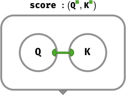
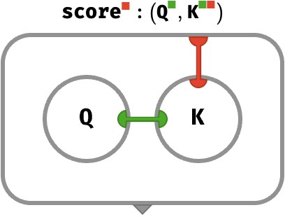
Current transformers model keys, queries, and values as vectors. To make it possible to score the relevance of a key-vector K to a query-vector Q, we demand they are vectors of the same shape ⟨K⟩. The simplest form of scoring is just the ordinary dot product between the two vectors, along the key axis:
          Q : ⟨K⟩
          K : ⟨K⟩
score(Q, K) : ⟨ ⟩

score(Q, K) ≡ Q ⊙ K
Single score #
In the simplest case, we can compare a single key with a single query, and we will obtain a scalar score. Let’s measure the score for query Q = [1, 0] against key K = [0, 1]:
score⎛⎡1  ⎡0⎞ = 0
     ⎝⎣0, ⎣1⎠
These vectors are orthogonal, and so the key is deemed irrelevant with a zero score. As another example, a query that matches the key gives a positive score:
score⎛⎡1  ⎡1⎞ = 1
     ⎝⎣0, ⎣0⎠
These examples involving single vectors correspond to the following rainbow circuit:
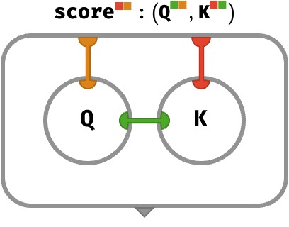
Sequence of scores #
We will be scoring every token in the input sequence against a single query – which means mapping the score operation over the novel N axis. Here is the type signature of the situation:
      Q     : ⟨  K⟩
         K  : ⟨N K⟩
score(Q, K) : ⟨N  ⟩
We obtain a sequence of scores, with one score for each key:
score⎛⎡1  ⎡⎡0 ⎡1 ⎡1⎞ = [0 1 1
     ⎝⎣0, ⎣⎣1 ⎣0 ⎣1⎠
The corresponding array circuit is as follows:
Notice that the red wire connects the key array to the exterior frame, representing that we will obtain N scalar scores, one for each key.
Parallel queries #
Hinting at the idea that we might execute multiple queries in parallel, let’s imagine a (potentially differently sized) sequence of queries applied to the sequence of keys:
      Q     : ⟨  K M⟩
         K  : ⟨N K  ⟩
score(Q, K) : ⟨N   M⟩
By ordinary rules of mapping, this produces a matrix of scores, containing the similarity of every pairing of a query with a key. Here’s a concrete example, which includes the score we saw for query [1 0], as well as the score for a new query [0 2]:
score⎛⎡⎡1 ⎡0  ⎡⎡0 ⎡1 ⎡1⎞ = ⎡[0 1 1
     ⎝⎣⎣0 ⎣2, ⎣⎣1 ⎣0 ⎣1⎠   ⎣[2 0 2
For now, though, we’ll concentrate on a single query at a time.
Softmax #
Let’s reconsider the example:
score⎛⎡1  ⎡⎡0 ⎡1 ⎡1⎞ = [0 1 1
     ⎝⎣0, ⎣⎣1 ⎣0 ⎣1⎠
Notice these scores do not add up to 1. Worse, dot products can be negative! To turn these scores into normalized weights that are appropriate in a weighted sum, we will apply the softmax operation, which for vector inputs is defined as xi = exp(xi) / sumj( exp(xj) ). The denominator is what normalizes the vector to ensure it sums to 1.
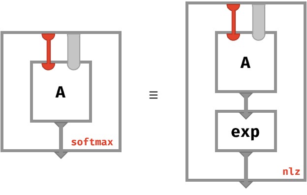
Here is the rainbow definition of softmax for a vector. Note we are parameterizing softmax with an axis so that it can operate on arrays of any arity and will only normalize across that particular axis.
A : ⟨■⟩ -> ℝ
softmax◆(A) : ⟨■⟩ -> ℝ
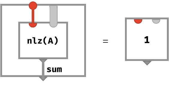
softmax◆(A) ≡ normalize◆(exp↑(A))
normalize◆(A) ≡ A /↑ sum◆(A)
We used an auxiliary function normalize. Let’s define it!
Defining normalize #
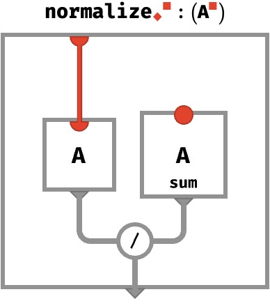
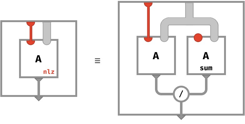
This definition involves mapping the exponential function over cells of A, and then applying the normalize operation, which ensures the result sums to 1. The cellwise definition for normalize is straightforward:
normalize◆(A) ≡ A /↑ sum◆(A)
Here, we show the array circuit for normalize:
If A has additional axes, they are carried over to the result. Again, this is the ordinary situation in rainbow algebra: operations “automap” over axes that are not explicitly part of their internal definition. Here, the thick gray wire represents all the axes of A except for red (if any). But let’s see the full picture for clarity:
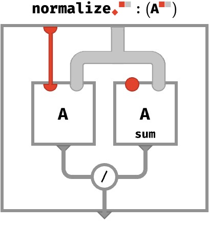
It can be hard at first to understand what normalizing a particular axis of a higher-arity array actually does! The answer is that it ensures that when we sum that axis, the resulting array will consist of all 1s. In the simple case of a vector, this ensures the resulting scalar is 1:
              V   = [1 2 3]

    normalize(V)  = [1/6 2/6 3/6]

sum(normalize(V)) = 1
Operating on a matrix, we see that red normalization only ensures that the red sum yields an array of 1s, but not so for the blue sum.
              M   = ⎡[1 2 3
                    ⎣[2 0 1

    normalize(M)  = ⎡[1/6 2/6 3/6
                    ⎣[2/3 0/3 1/3

sum(normalize(M)) = [1 1
sum(normalize(M)) = [5/6 2/6 5/6
The equation that normalize obeys with respect to sum is then (stated for any axis, where 1|A| is the constant array of 1s of A’s shape):
sum◆(normalize◆(A)) = 1|A|
In circuit form, this is:
Defining softmax #
With those axis semantics explained, we’ll go on to define softmax itself. First, we’ll use the following abbreviation:
Generic softmax #
The fully generic diagram of softmax◆(A) can then be written as:
Attention weights #
To utilize softmax to obtain attention weights, we wish to normalize over the sequence axis, since we want the total weight across the sequence to be 1.
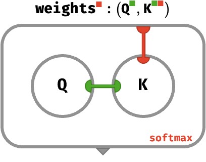
Here is how we use it to compute the attention weights for a single query applied to sequence’s worth of keys:
        Q     : ⟨  K⟩
           K  : ⟨N K⟩
weights(Q, K) : ⟨N  ⟩

weights(Q, K) ≡ softmax◆(score(Q, K))
              ≡ softmax◆(Q ⊙ K)
Applying this operation to our original example query, we arrive at the following result:
weights⎛⎡1  ⎡⎡0 ⎡1 ⎡1⎞ = softmax([0 1 1) = [0.16 0.42 0.42
       ⎝⎣0, ⎣⎣1 ⎣0 ⎣1⎠
We now have a sequence worth of weights which can be used to perform a weighted sum! That’s what we’ll define in the next section.
Previewing the fact that our definitions can be mapped to operate in parallel over a novel axis, let’s compute the weights for two queries in parallel:
weights⎛⎡⎡1 ⎡0  ⎡⎡0 ⎡1 ⎡1⎞ = softmax⎛⎡[0 1 1⎞ = ⎡[0.16 0.42 0.42
       ⎝⎣⎣0 ⎣2, ⎣⎣1 ⎣0 ⎣1⎠          ⎝⎣[2 0 2⎠   ⎣[0.47 0.06 0.47
The signature of this mapped usage of weights is:
        Q     : ⟨M   K⟩
           K  : ⟨  N K⟩
weights(Q, K) : ⟨M N  ⟩
Weighted sum #
Next, we will see how to sum the value vectors, weighted by their softmax-normalized scores, which were derived by comparing the query vector to the key vectors. In this sum, a value vector whose corresponding key vector was deemed more similar to the query will be weighted more highly in the sum. Note that the value vectors need not have the same size as the key and query vectors, so we’ll use the novel axis V for these value vectors.
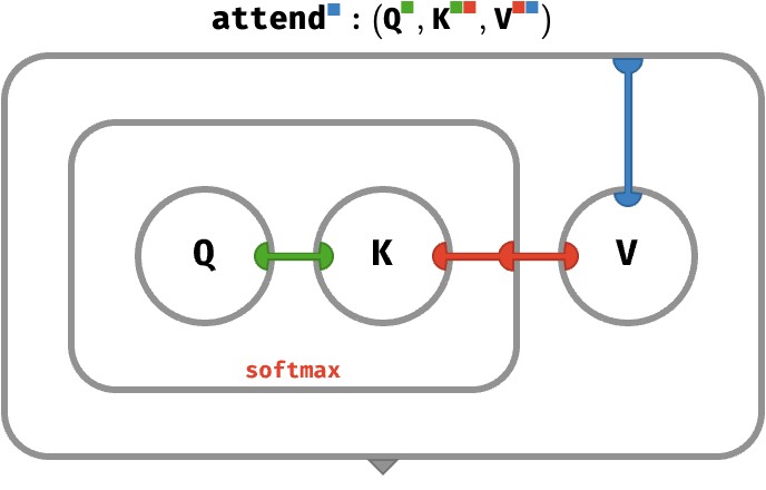
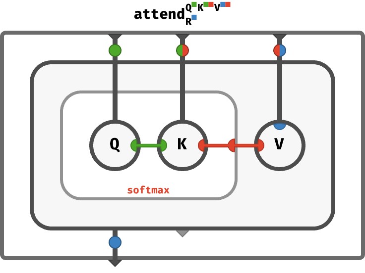
We’ll encapsulate all this in an operation called attend, which takes a query vector, a key matrix, and a value matrix. It computes the weights, and uses these to perform a weighted sum of values:
       Q        : ⟨K    ⟩
          K     : ⟨K N  ⟩
             V  : ⟨  N V⟩
attend(Q, K, V) : ⟨  N V⟩

attend(Q, K, V) ≡ weights(Q, K) ⋅ V
                ≡ softmax(Q ⊙ K) ⊙ V
To understand this definition, first notice that if we have a sequence of normalized weights W and a sequence of V-vectors V, the following circuit will perform a weighted sum, weighting each element of the sequence V by its corresponding weight in W:
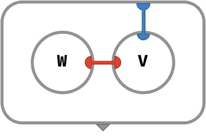
Since the weights are W = weights(Q,K), we can substitute the subcircuit for computing these weights to yield the full circuit:
You can think of attend as performing a kind of database lookup. Imagine holding the matrices K and V fixed. Then attend defines a transformation from a query K-vector to a result V-vector. Hence, the K and V matrices make up the two columns of a database table with N rows, where Q is the query made against the first column in this database, with the second column yielding the results of the query, summed according to the similarity of each match.
Abstracting #
So far we have a sort of hard-coded circuit in which the keys, queries, and values are embedded in the circuit rather than being supplied as inputs. To rectify this, we need to abstract. This is much like going from a stand-alone piece of code, to a function that takes the needed data as inputs. (A similar thing happened in the section on perceptrons.)
The way abstraction works in array circuits is via the bubbles that we discussed in the section on closures. Instead of Q being an internal vector that lives inside the circuit, we’ll pipe Q in as a vector-valued input, and pipe the result out as a vector-valued output. The dark gray wires are array-valued-wires that carry arrays around. This is essentially treating array programs as higher-order functions that transform functions (arrays) into other functions (arrays).
Here we go!
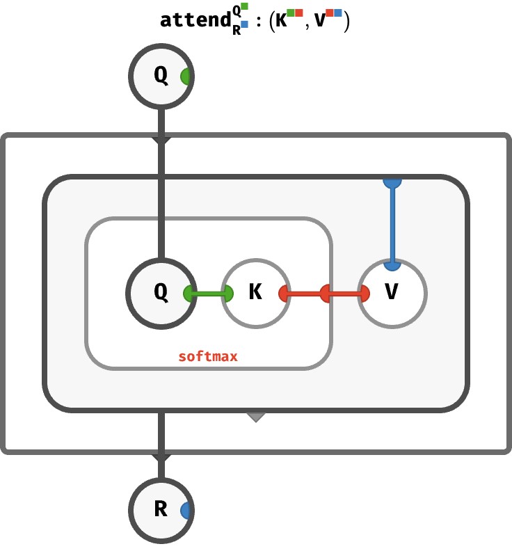
Notice that the input K-vector – the query vector – is piped into an interior bubble with a green port. Likewise, the outer interior bubble (the result of the query) has a single blue port, and is piped to the output ■-vector – the result vector.
Decorating array wires #
The bubbles outside the attend array in the circuit above are really just naming the inputs and outputs, and allowing us to see what ports these array-valued inputs and outputs have. This isn’t ideal. A less noisy approach is to decorate the interior wires with little medallions that indicate what ports are available on the arrays that these wires carry. Here, we see the input wire carries a K-vector (the query) and the output wire carries a V-vector (the result):
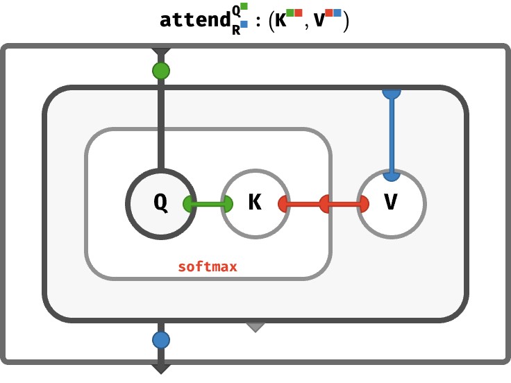
At this point, we’ve defined a circuit that represents a function which maps a query input K-vector to a result output vector V-vector. The sequence of keys and values that the query is made against are held fixed inside the network, which is why K and V still appear in brackets in the type signature. But we can go further to abstract those too to become explicit inputs!
Abstracting over keys and values #
We can repeat the same trick to abstract over the matrices K and V as well, so they go from being interior arrays to explicit array-valued inputs:
Took a moment to sanity-check the medallions. Done? The query input is a K-vector, key input is KN-matrix, the values input is a VN-matrix, and the result output is a V-vector.
Tokens, queries, keys, and values #
We’ve described how the attend function can compare a single query vector against a sequence of key and value vectors to obtain a result vector.
Let’s summarize the kinds of vector in play – realizing that we’re dealing sequences of such vectors, aka matrices with a red axis:
| z | z | z | z |
|---|---|---|---|
| shape | name | description | |
T |
⟨T⟩ |
token vector | vector used to derive Q, K, V |
Q |
⟨K⟩ |
query vector | query applied against all keys in this round |
K |
⟨K⟩ |
key vector | key observed by all queries in this round |
V |
⟨V⟩ |
value vector | value used in all weighted sums |
R |
⟨V⟩ |
result vector | result of weighed sum |
But where do the query, key, and value vectors actually come from? And what do we do with the result vector? This is where learned parameters come in.
In the transformer architecture, in each round of self-attention, we will use each token vector T to produce one of these Q, K, and V vectors via learned perceptrons.
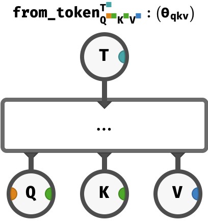
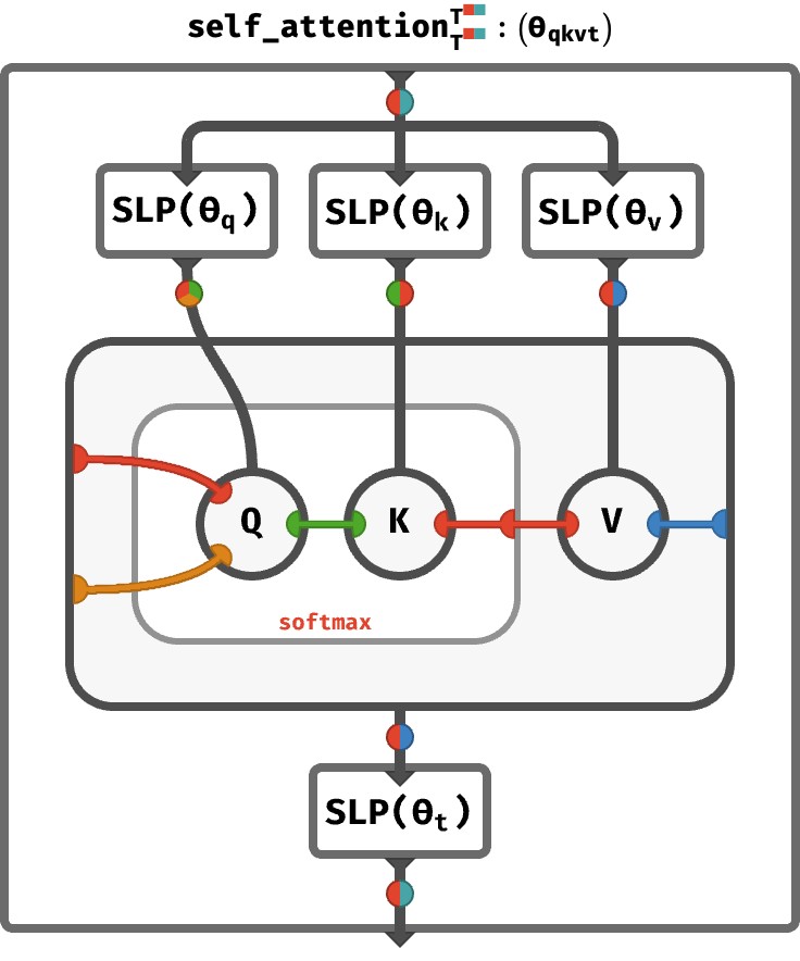
We’ll encapsulate this process of computing Q, K, and V vectors from a T vector using a single function called from_token, which contains one perceptron to produce each vector:
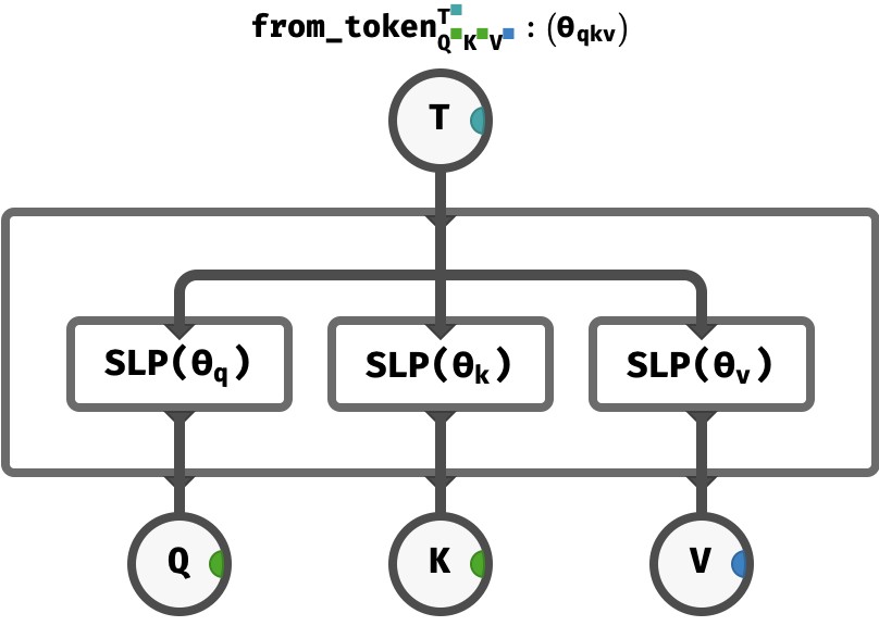
Notice the internal weights and biases of the all three perceptrons are gathered together as the parameter ϴqkv of from_token as a whole. These arrays will trained by gradient descent when the full transformer is exposed to training data.
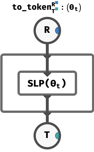
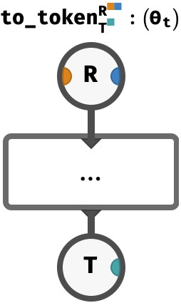
The function from_token will give us the ingredients we need to perform attention. But once attention has been performed, we need to processes the result of attention (a V-vector) back into a T-vector, which we do via a to_token function, containing a single perceptron:
Sequences of tokens #
By mapping from_token over the sequence axis, we can process in parallel a sequence of tokens to produce a sequence of query, key, and value vectors:
This happens automatically via axis genericity.
The sandwich #
At this point, we can feed these matrices to attend, which recall has this signature and definition:
       Q        : ⟨K    ⟩
          K     : ⟨K N  ⟩
             V  : ⟨  N V⟩
attend(Q, K, V) : ⟨  N V⟩

attend(Q, K, V) ≡ weights(Q, K) ⋅ V
                ≡ softmax(Q ⊙ K) ⊙ V
You might object that attend expects a single query vector and produce a single result vector. Whereas our from_token gives us a sequence of queries.
But we can also map attend, so that it takes a sequence of queries and produces a sequence of results.
And similarly we can map to_token so that it transforms this sequence of result vectors into a sequence of token vectors. Putting this all together, we have a kind of “sandwich”, with attend forming the meat (or your choice of vegan cheese perhaps):
That’s it! That’s one round of self-attention. Transformers apply self-attention multiple times, with the final results being the token vectors at the very end. These can be used to make a prediction of the next token or for other tasks.
A bit more detail #
Now, you might complain that we’ve hidden some of the complexity inside the attend, from_token, and to_token functions. Of particular interest: the sequence axis is being used in two different ways: a sequence of queries is being provided to attend, but this sequence axis is being treated differently to the (identical) sequence axis present in the key and value arrays. So let’s expand the definition to see what exactly is going on:
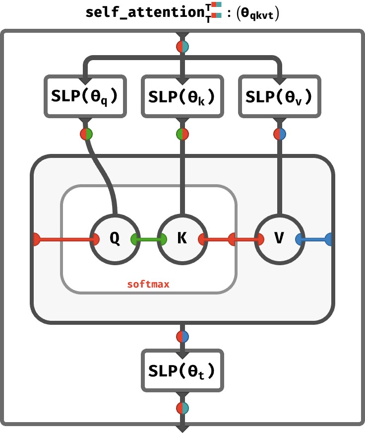
Notice that the sequence axis of the key and value arrays participates in the softmax operation (you can see it is connected to the right-hand red port of the softmax box). In contrast, the sequence axis of the query array appearing on the left-hand port passes straight through the softmax, meaning it is simply used to index the entire result vector. This illustrates that each the n‘th result is derived from the n‘th query.
The fact that there are two separate red wires in the attention part of the circuit is why this is called self-attention. The sequence of queries (indicated by the left red wire) and the sequence of keys and values (indicated by the right red wire) are derived from the same sequence, because they’re both red wires! In words: the sequence is attending to itself!
Multi-head attention #
What we’ve described is the simplest form of self-attention. Each token makes precisely one query. But it is very powerful to allow a token to make H distinct queries, yielding H distinct results, that are then combined in a more sophisticated way to produce a final token vector. This extension is extremely easy to express in rainbow terms.
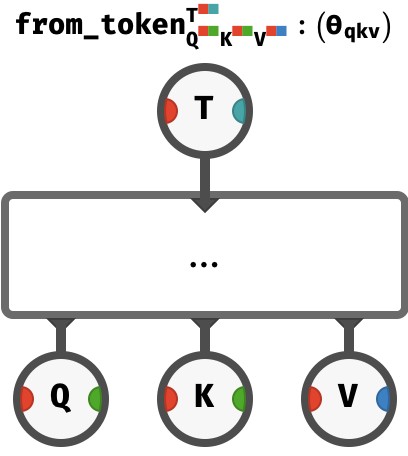
We first define from_token to produce H distinct queries:
The only change from before is that the output Q array has an additional H axis.
I’ve elided the actual circuit. We could implement this new signature of from_token by using H distinct perceptrons to produce Q, one for each “attention head”. But in fact this is not necessary, since the perceptrons in rainbow arrays can emit matrices just as easily as they emit vectors, if the corresponding weight and bias arrays have an additional H axis.
Similarly, we redefine to_token to accept H distinct results:
In practical terms we can achieve this by reshaping the input HV-matrix into a vector and applying an SLP to obtain a T-vector. Again, we won’t show the actually circuit to do this, since it is a minor technical detail.
We’ve updated the bread to be multi-head, what about the filling? Luckily, the semantics of rainbow mapping ensure that attend will execute these H distinct queries in parallel. Let’s slap together the full sandwich to see how this works:
An unforgettable luncheon!
The full stack #
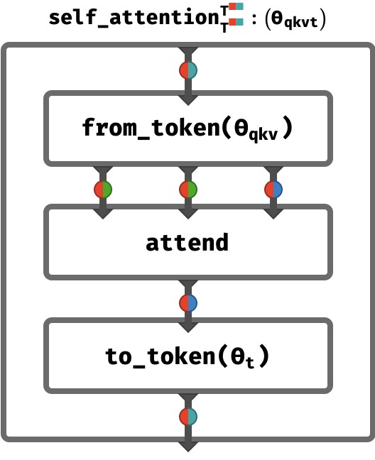
Having described the core action of self-attention, we can now summarize the full transformer data flow.
Firstly, while we’ve described the essence of self-attention, a small amount of post-processing is still involved. We’ll encapsulate all these steps in a single round function, shown below. Note that transformer architectures can vary in what they do here, so we’ve simplified the contents of this step a bit.
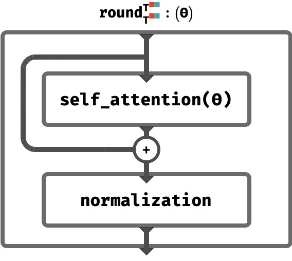
Here, the results of self-attention are added the previous token vectors, rather than replacing them – this is known as a residual network. Additionally, a form of normalization is used that tries to keep the norms of the token vectors constant as we go deeper into the network. As these don’t relate to attention, we won’t focus any further on the details here.
All that remains is to apply multiple rounds in series, successively transforming the sequence of token vectors:
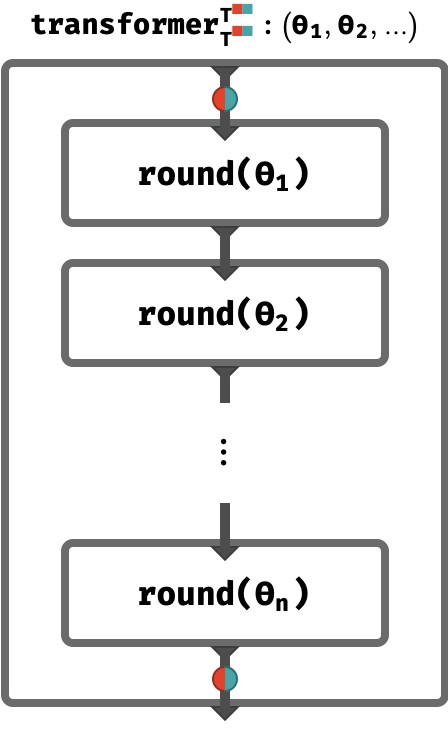
Notice that the entire transformer has internal arrays ϴi each of which denote the internal arrays ϴq, ϴk, ϴv, ϴt associated with the perceptrons in that round. These are typically all distinct arrays that are trained by gradient descent.
Wrapping up #
After many rounds of self-attention, the final token vector sequence we obtain can somehow encode the meaning of the sequence – as long as the training set has forced the network to distill such a meaning in order to perform the task. Depending on the task, these vectors can be used in several ways.
For predictive tasks, it is possible to process the entire ■■-matrix to produce a fixed dimensional vector for the task.
For autoregressive networks like ChatGPT, in which the task is to predict the next token, we instead use the (final) n’th token ■-vector to obtain a prediction for the as-yet-unseen next token in the sequence. In practice, some additional details intervene: the method of teacher forcing is used to train autoregressive networks, in which a process called causal masking applied during the self-attention steps ensures that we can obtain gradients from the full set of sequence prefixes [t1], [t1 t2], [t1 t2 t3], etc. using only a single evaluation of the transformer on the full sequence [t1 t2 t3 … tn], but we leave this detail to other sources to explain.
And that’s it. Congratulations on making it to the end of a multi-course meal!
Takeaways #
Advantages #
Rainbow array algebra keeps semantic meaning (e.g. sequence position, colour channel, batch number, time, feature dimension) attached to array axes, and abandons axis order. This leads to fewer primitive operations and greater clarity of the meaning of an particular operation deep inside an array program, because the semantic context is carried along.
Additionally, we can use various notational conveniences like half-framing to make higher-arity arrays easier to read and write. Since order does not matter, we can arrange lay these axes out visually in whatever way improves clarity.
Axis genericity means that rainbow operations automatically scale up to include additional novel axes with no additional complexity. We saw a nice practical example of this in the extension of the transformer architecture to [[[multi-head attention:#multi-head-attention]], otherwise a somewhat obscure detail of transformers.
In my view, rainbow arrays represent the future of array programming – or at least one incarnation of it. Indeed, some deep learning researchers are currently pushing for labeled axes to become the standard approach. As array programs weave themselves into more critical parts of our global software infrastructure, making their operation more transparent and debuggable is a noble goal.
Future directions #
Future posts will explore some interesting aspects of rainbow array algebra. Here’s a list of questions I hope to explore, in no particular order:
-
What is the diagrammatic formulation of rainbow array operations in terms of part / key dataflow? For example, broadcasting is deleting a flow, and taking the diagonal (which we didn’t describe in this post) is copying a flow. How do these flows compose?
-
Along the same vein: what are the formal composition properties of rainbow arrays in terms of category theory?
-
What is the right design for a software library that implements these ideas to their full extent? Even though they focus on arrays, the underlying ideas are about higher-order functional programming, so can they subsume more traditional, functional programming constructs?
-
What are the connections to hypergraph rewriting? In particular, graphs have adjacency matrices; hypergraphs have adjacency hypermatrices.
Thanks #
- Thanks to Bruno Gavranović for valuable feedback on the transformer section.
References #
There is some great prior work that propose rainbow-like approaches to array programming, going largely under the rubric of “named axes”. I intend to say more about how this post connects to prior work, but for now, here are some key references:
-
Alexander Rush discusses the myriad problems with existing multidimensional array programming APIs and proposes solutions in a series of blog posts “Tensors considered harmful”.
-
Chiang, Rush, and Barak have proposed a “Named Tensor Notation” to clarify the exposition of deep neural network architectures in published literature.
-
Maclaurin, Paszke et al. have made the functional perspective on array programming a core part of their Dex Haskell library.
-
Hoyer et al have pursued these ideas for a long time under the aegis of the XArray project.
-
Lastly, my colleagues and I discuss similar ideas in our paper “Heaps of Fish”.
-
For more details about the transformer architecture, the original paper “Attention is all you need” is all you need.