Classical array algebra #
Introduction #
The goal of this first post is to clearly explain what multidimensional arrays are, and how they are manipulated in classical array programming. To this end I’ll introduce some notational devices for writing multidimensional arrays and expressing their operations. I’ll set out a general mathematical framework for reasoning about these arrays and their operations that is independent of the details of particular frameworks like NumPy or Torch.
The perspective I’m promoting here is to think about arrays as functions from indices to values. This view is starting to be adopted in practice – it’s a key design principle of the deep learning research language Dex. The “arrays as functions” perspective also naturally leads us to a kind of diagrammatic notation that is inherited from category theory, though I won’t elaborate on those connections here.
The followup post builds on this foundation to present an alternative paradigm called rainbow array algebra. In that post, I draw on color as a way of labelling array axes, instead of the traditional way we use a fixed axis order. But the principle is the same as named axes that are proposed in the Sasha Rush’s excellent “Tensors considered harmful”. In my view, this alternative paradigm simplifies and unifies many of the constructions we’ll see below, and offers a better foundation for array programming in the coming decades.
Array programming #
Array programming, meaning computation on multidimensional arrays, is a foundational component of signal processing, data science, data visualization, and machine learning. Popular software libraries for doing array programming include Numpy, Scipy, R, Pandas, Torch, Tensorflow, JAX, XArray, and Julia. But the first array language was arguably Ken Iverson’s APL, which has modern descendents like K, J, and BQN.
Multidimensional arrays are used to represent time series, multimedia data, sensor measurements, system logs, financial transactions, medical outcomes, user behavior, neural network activity and a large number of other domain-specific data.
Software programs that manipulate arrays I’ll call array programs. We’ll aim to capture what array programs are doing at a conceptual level. The target audience is broad, including software practitioners interested in mathematical formalisms as well as mathematicians interested in array programming. It is unavoidable that some details will be redundant for some readers – please skip sections as appropriate.
Abstract nonsense #
The constructions in array algebra can be understood within the framework of category theory. We won’t elaborate on this connection here, and leave this to a future blogpost. Briefly, arrays themselves can be seen as morphisms in a Cartesian closed category, with objects being part spaces and the Cartesian product of part spacing forming key spaces. This makes array circuit into string diagrams, which when “framed” exhibit array programs as lambda abstractions. The existence of an internal hom is what enables us to represent arrays themselves as values, see nesting. Our bubble notation resembles Ghica and Zanasi’s notation, see also Baez’s bubble and clasp notation.
Basic theory #
Core concepts #
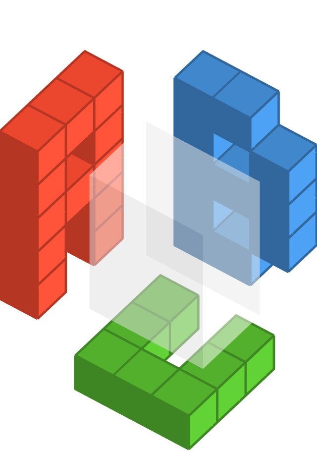
At a high level, an array is a container of values. These values are organized in a particularly regular way – along axes. The number of axes of an array – the arity of the array – largely determines how the array can be processed and combined with other arrays.
Here’s a simple visual depiction of arrays with 0 through 3 axes, along with the shapes that describe the dimensions or sizes of the successive axes.
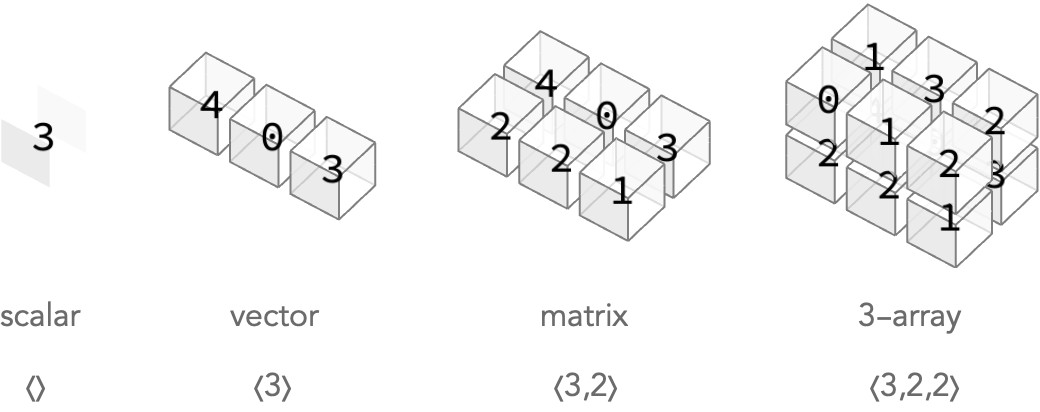
Each of the cubes above is called a cell, and contains a single value – integers in these cases.
The arity counts the number of axes of an array: a scalar has no axes, a vector has one axis, a matrix has two axes (rows and columns), etc. An array with n axes will be called an n-array.
Terminology #
Let’s focus on a matrix – an array with two axes – to illustrate our terms.
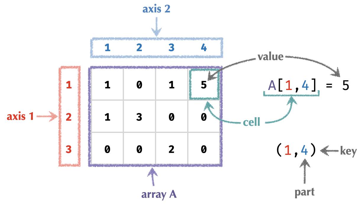
The terms we’ll use for the rest of this post are defined below:
| z | z |
|---|---|
| array | a collection of cells |
| cell | a slot in an array labeled by a key filled with a value |
| key | position of a cell in an array a tuple of parts |
| axis | a label for a part an integer in 1..n |
| value | the contents of a cell |
Notation #
As the vast majority of programming languages do, we’ll use the convention of nested lists to write arrays with multiple axes. More deeply nested lists correspond to higher-numbered axes.
For example, the 3-vector V = [1 2 3] has one axis and has three cells, each containing an integer value.
A 2-row, 3-column matrix M = [ [1 2 3] [4 5 6] ] has two axes (rows, columns) and contains six cells. Typically, these axes are arranged with the first axis vertically and the second horizontally:
M = [[1 2 3]
     [4 5 6]]
Colour coding #
We can use colour coding to help distinguish how lists at different levels of nesting correspond to different axes of the array:
M = [[1 2 3]     axis 1
     [4 5 6]]    axis 2
Framing #
In addition, we will extend the brackets to span multiple rows, making it clearer how the lists contain more deeply nested lists via “framing”:
M = ⎡[1 2 3]⎤
    ⎣[4 5 6]⎦
Part labels #
Typically, the successive elements in each nested list […] correspond to the cells at parts 1,2,3…, increasing to the right if the list is arranged horizontally, and increasing down if arranged vertically. We can make this more explicit by labelling the parts of each axis:
    1 2 3
1 ⎡[1 2 3]⎤
2 ⎣[4 5 6]⎦
This labelling will become necessary rather than optional when part spaces are not of the form 1..n, but some other set without a defined order.
Multiple axes #
At this point we have run out of dimensions on the page, but we can lay out more axes as we see fit for aesthetic purposes:
⎡ ⎡[1 1]⎤ ⎡[0 1]⎤ ⎡[0 0]⎤ ⎡[1 1]⎤ ⎤
⎢ ⎢[0 1]⎥ ⎢[0 1]⎥ ⎢[0 0]⎥ ⎢[0 0]⎥ ⎥
⎣ ⎣[0 0]⎦ ⎣[0 0]⎦ ⎣[0 1]⎦ ⎣[0 0]⎦ ⎦

         1st axis; size 4
         2nd axis; size 3
         3rd axis; size 2
Half-framing #
We can additionally achieve a more compact presentation by eliding the right hand frame. Here we show the half-framed version of the 3-array from earlier:
⎡⎡[1 1 ⎡[0 1 ⎡[0 0 ⎡[1 1
⎢⎢[0 1 ⎢[0 1 ⎢[0 0 ⎢[0 0
⎣⎣[0 0 ⎣[0 0 ⎣[0 1 ⎣[0 0

    1st axis; size 4
    2nd axis; size 3
    3rd axis; size 2
We’ll mostly use this variant of framing notation.
Layout #
In fact, we can choose each axis to be horizontal or vertical independently. For example, the vector V = [ 1 2 3 ] can be written in both of these ways, they are equivalent:
         ⎡1
[1 2 3 = ⎢2
         ⎣3
For us, there is no such thing as a column vector or row vector – such terms only have meaning when talking about how we can deconstruct a matrix into a vector-of-vectors – which we will discus in the section about the nest operation.
Similarly, there are four equivalent ways of writing the matrix M = [ [1 2 3] [4 5 6] ], depending on whether we choose to lay out the each of the two axes vertically or horizontally:
⎡⎡1 = ⎡⎡1 ⎡4 = ⎡[1 2 3 = [[1 2 3 [4 5 6
⎢⎢2   ⎢⎢2 ⎢5   ⎣[4 5 6
⎢⎣3   ⎣⎣3 ⎣6
⎢⎡4
⎢⎢5
⎣⎣6
The third layout is considered canonical, because it matches the traditional interpretation of the first axis of a matrix as enumerating the rows, and the second axis the columns.
Part and key spaces #
A part space is typically a set of the form 1..n ≡ {1,2,…,n}, allowing us to write cells horizontally or vertically in order without resorting to explicit part labels.
A key space is the space of tuples formed from these part spaces.
For an n-array, a key space can be denoted by a shape written ⟨s1,s2,…,sn⟩, which refers to the n-ary Cartesian product:
⟨s1,…,sn⟩ ≡ { (p1,…,pn) | pi ∈ 1..si }
For example, a matrix with 3 rows and 2 columns has shape ⟨3,2⟩, which is the Cartesian product of part spaces 1..3 and 1..2 for the first and second axes respectively:
⟨3,2⟩ ≡ { (r,c) | r ∈ 1..3, c ∈ 1..2 }
      = { (1,1), (1,2), (2,1), (2,2), (3,1), (3,2) }
As a degenerate case, a scalar array has the shape:
⟨⟩ = { () }
So a scalar has only one cell – with position () – and hence only one value!
We have already seen part spaces that aren’t consecutive natural numbers – the total order on ℕ is usually not used or needed except for easy display or storage.
Arrays as functions #
We can see an array A as a function from its key space to its value space. Arrays are just lookup tables, to use computer science terminology. Array algebra is then the algebra that manipulates lookup tables.
An \(n\)-array is just a function of \(n\) variables. Or equivalently, a unary function with a single argument that is an \(n\)-tuple. The cell value A[1,2,3] is shorthand for function application A( (1,2,3) ):
A[…] ≡ A( (…) )
In the next post, we will see how rainbow arrays replace this tuple with a data-structure called a record.
Array circuits #
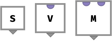
Since arrays are just functions, it will be helpful to depict how them graphically using diagrams called array circuits. These diagrams show the array as a box, with ports on the top that represent the parts of the key space, and a single port on the bottom that represents the value. The ports are labeled in order from left to right.
Here we show a scalar array S, a vector array V, and a matrix M:
When we “wire” together several of these arrays into a circuit, we can represent how simple arrays can be combined into more complicated ones. While more complex examples will be shown in later sections, here we show how a function f:V->V can be applied to the value of each cell of a matrix M:
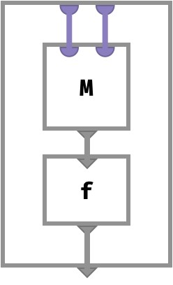
This array derived from M and f is also a matrix, since the entire outer frame has two input key ports and one output value port.
It’s worth emphasizing again that the left-to-right order of ports in each box is what defines the axis order of the corresponding arrays.
Table of arrays #
This table shows arrays of increasing arity.
| arity | nested form | shape | example keys and values |
|---|---|---|---|
| 0 (scalar) | 9 |
⟨⟩ |
() -> 9 |
| 1 (vector) | [9 1 5 |
⟨3⟩ |
(3) -> 5 |
| 2 (matrix) | ⎡[9 1 5 |
⟨2,3⟩ |
(1,1) -> 9 |
| 3 | ⎡⎡[0 1 |
⟨3,2,2⟩ |
(1,1,1) -> 0 |
| 4 | ⎡⎡⎡[0 0 ⎡[1 2 |
⟨3,2,2,2⟩ |
(1,1,1,1) -> 0 |
Array applications #
In this section we will illustrate some basic applications of multidimensional arrays from several different fields. The goal is to give us a diverse set of examples which will make usefulness of array algebra operations clearer. If you’re familiar with such uses of multidimensional arrays, please skip ahead to the section on primitive operations.
Text #
Text manipulated by a computer is usually represented with a so-called string, a data structure in which the first symbol of the text is taken to be at position 1 and the last symbol at position N. The symbols themselves are elements from some fixed alphabet. For ASCII text, this alphabet consists of 255 symbols, containing the Roman alphabet, punctuation, and a few non-Roman letters. The Unicode standard introduces a vastly largely alphabet that covers practically all know written symbols, and forms the backbone of modern text processing today. How such large alphabets are compactly encoded to fit as sequences of bytes will not concern us – we will view strings as logical data structures that store symbols at consecutive integer positions:
| axis | meaning | part space |
|---|---|---|
1 |
position of symbol in string | 1..N |
Strings of length N therefore have the type:
S : ⟨N⟩ -> U
For example, the string hello world can be seen as 1-array, where the value space U is the set of Unicode symbols: U = {a, b, c, d, … }:
S = [h e l l o w o r l d]
Histograms #
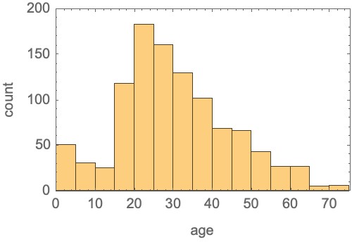
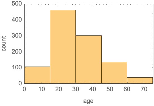
Histograms offer a useful statistical summary of numeric data. Let’s take as an example the ages of passengers of the Titanic at the time of its fateful accident. The ages of 1046 passengers are known. We can summarize these by counting the number of passengers that fall into “bins” of age 0-5, 5-10, 10-15, etc:
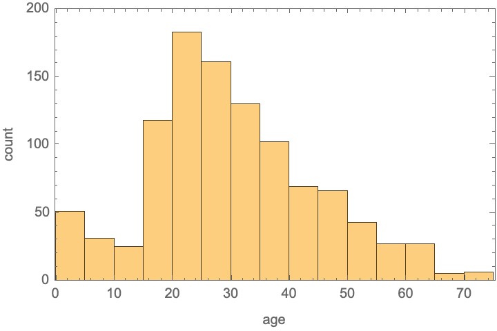
Logically, we can see the histogram as an array with one axis whose part correspond to the age bins. Formally, these bins are intervals [l,u) mentioning a lower and upper bound. For the Titanic example, we chose bins B = {[0,5), [5,10), …}, etc.
| axis | meaning | part space |
|---|---|---|
1 |
bin | B = {[l1,u1), [l2,u2), …} |
The value space is the set of natural numbers ℕ, because each cell contains a count of how many passengers were in that bin. Therefore this sort of one-dimensional histogram is an array of type:
H : ⟨B⟩ -> ℕ
In the case of the titanic dataset, this histogram array is given by:
H = [51 31 25 118 183 161 130 102 69 66 43 27 27 5 6]
(Even though the part space is not of the form 1..N, we can suppress the part labels, since the bin intervals have a natural order.)
Discrete probability distributions #
First, let’s consider a discrete probability distribution over a set of symbols. This could represent the probabilities that a piece of text written using a fixed alphabet A will be a followed with a particular symbol from that alphabet. This is a method used by generative text models like an ChatGPT, for example.
| axis | meaning | part space |
|---|---|---|
1 |
symbol from a fixed alphabet | A = {a,b,c,d,…} |
Therefore, such an array is a simply a vector of real numbers between 0 and 1, with the constraint that the sum of all these probabilities must sum to 1. We will denote this value space with 1 ≡ [0,1] ≡ { p ∈ ℝ | 0 ≤ p ≤ 1 }:
P : ⟨A⟩ -> 1
Let’s consider an example for the standard 26-letter Roman alphabet, in which the predicted next symbol is most likely to be a, but there is some probability to be e or f:
      a  b  c  d  e  f  g  h  i  j  k  l  m  n  o  p  q  r  s  t  u  v  w  x  y  z
P = [.6 .0 .0 .0 .2 .2 .0 .0 .0 .0 .0 .0 .0 .0 .0 .0 .0 .0 .0 .0 .0 .0 .0 .0 .0 .0
Here, the parts are not consecutive integers but symbols from the alphabet, and hence we label each cell with that symbol. Heed this example: part spaces can be logically quite interesting sets (in this case the set of Roman letters) that have no natural correspondence with integers!
Contingency tables #
A vivid class of examples comes from experimental medicine. Let’s imagine a RCT (randomized controlled trial) in which we are trying to decide which (if either) of two medicines for the common cold is effective. We will treating a cohort of 150 patients using one of the two medicines, or no treatment at all. After splitting the patients into three equally sized and matched groups of size 50, we apply the relevant treatment to each patient, and then observe their clinical outcome after 3 days, which we will classify as recovered or ill.
We can represent these using two axes of an array:
| axis | name | meaning | part space |
|---|---|---|---|
| 1 | T |
treatment | {none, medicine 1, medicine 2} |
| 2 | O |
outcome | {recovered, ill} |
The value space of the array will be a natural number ℕ representing how many patients experienced a particular outcome when given a particular treatment. Therefore, these observations can be recorded in array:
C : ⟨T,O⟩ -> ℕ
Here is an example such array, which is more commonly called a contingency table:
        no  m1  m2
C = ⎡ [ 10  28  13   recovered
    ⎣ [ 40  22  37   ill
Grayscale images #
Images are ubiquitous artefacts in computing.
They can be represented as arrays of numbers that indicate the coloured light intensity in each two-dimensional location on the image, or pixel (which is derived from picture element).
The simplest case is a grayscale image, where each pixel can be described by a real number between 0 and 1 that represents its brightness. The number 0 means no light (black) and 1 means full light intensity (white).
We can represent such a grayscale image of width W and height H as a matrix whose cells contain pixels. The first axis represents where a pixel is vertically on the image, ranging from 1 for the top of the image to H for the bottom, and the second axis represents where a pixel is horizontally, ranging from 1 for the left to W for the right:
| axis | name | meaning | part space |
|---|---|---|---|
| 1 | Y |
vertical position of a pixel | 1..H |
| 2 | X |
horizontal position of a pixel | 1..W |
The value of such an array is a light intensity from the value space 1, making an image array into the following function:
I : ⟨H,W⟩ -> 1
As an example, let’s consider the black letter "F" as depicted by a grayscale image that measures 5 pixels by 3 pixels:
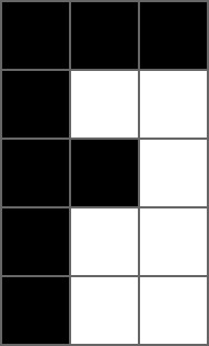
The corresponding image array is:
    ⎡[0 0 0
    ⎢[0 1 1
I = ⎢[0 0 1
    ⎢[0 1 1
    ⎣[0 1 1
We can see the pattern of 0s, which correspond to black pixels, forms an "F".
Colour images #
The situation with image arrays gets a little more complicated with colour images, because a coloured pixel requires three intensity values to represent, corresponding to light intensity combination of red, green, and blue light. These individual values are often referred to as subpixels.
Here is an example of how such mixtures of light intensity correspond to particular coloured pixels:
     r g b        r g b        r g b
■ = [0 0 0   ■ = [1 0 0   ■ = [1 1 0
■ = [½ ½ ½   ■ = [0 1 0   ■ = [0 1 1
□ = [1 1 1   ■ = [0 0 1   ■ = [1 0 1
To store all these subpixels in an array, we require 3 axes. A common ordering for these axes is the CYX convention, in which the so-called colour channel is the first axis:
| axis | name | meaning | part space |
|---|---|---|---|
| 1 | C |
colour channel of a subpixel | {R,G,B} or {1,2,3} |
| 2 | Y |
vertical position of a subpixel | 1..H |
| 3 | X |
horizontal position of a subpixel | 1..W |
This makes a colour image array a function of the form:
I : ⟨3,H,W> -> 1
Let’s examine the raw data underlying the following colour image that measures 5 pixels height by 4 pixels wide:
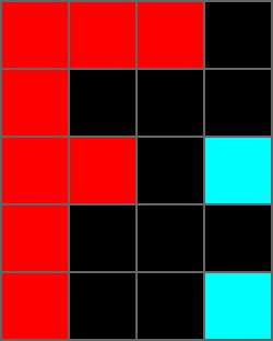
In this image, most pixels are black, which corresponds to light intensity values of 0 for all colour channels. The pixels for the "F" are red, with an intensity of 1 for the red channel and 0 for the others. The pixels for the ":" are aquamarine, with an intensity of 1 for the blue and green channels and an intensity of 0 for the red channel.
Let’s visualize all these intensities in a three-dimensional plot. Subpixels are tinted with the colour indicating which channel they correspond to. The black pixels are hidden for clarity:
Represented as an array using the CYX axis ordering convention, we have:
          r         g         b
    ⎡⎡[1 1 1 0 ⎡[0 0 0 0 ⎡[0 0 0 0
    ⎢⎢[1 0 0 0 ⎢[0 0 0 0 ⎢[0 0 0 0
I = ⎢⎢[1 1 0 0 ⎢[0 0 0 1 ⎢[0 0 0 1
    ⎢⎢[1 0 0 0 ⎢[0 0 0 0 ⎢[0 0 0 0
    ⎣⎣[1 0 0 0 ⎣[0 0 0 1 ⎣[0 0 0 1
Here, we can see the "F" in the pattern of 1s and 0s in the first channel, and similarly for the ":". Notice that in CYX convention a colour image is essentially three separate grayscale images representing the red, green, and blue “layers” that are combined to form the final colour image.
Another common axis ordering convent is YXC, in which the colour channel is instead the 3rd axis, corresponding to a shape ⟨5,4,3⟩. In this convention, we can instead see the array as resembling a matrix whose cells contain coloured pixels:
       r g b  r g b  r g b  r g b
    ⎡[[1 0 0 [1 0 0 [1 0 0 [0 0 0
    ⎢[[1 0 0 [0 0 0 [0 0 0 [0 0 0
I = ⎢[[1 0 0 [1 0 0 [0 0 0 [0 1 1
    ⎢[[1 0 0 [0 0 0 [0 0 0 [0 0 0
    ⎣[[1 0 0 [0 0 0 [0 0 0 [0 1 1
Here, the inner 3-vectors correspond to pixels as follows:
     r g b
■ = [1 0 0
■ = [0 0 0
■ = [0 1 1
If we display these inner 3-vectors in pixel-like form, the underlying image is clearer:
⎡[■ ■ ■ ■
⎢[■ ■ ■ ■
⎢[■ ■ ■ ■
⎢[■ ■ ■ ■
⎣[■ ■ ■ ■
Voxel images #
Modern medical devices such as MRI machines and CAT scanners can make three-dimensional scans of the human body. In these applications, the data that is obtained measures properties such as density or blood flow through a dense grid of small three-dimensional volumes of biological tissue. The term voxel is used for these measurements, where voxel derives from volume element.
Here is such an MRI scan of a knee joint, representing a grid of 128 by 128 by 128 voxels:
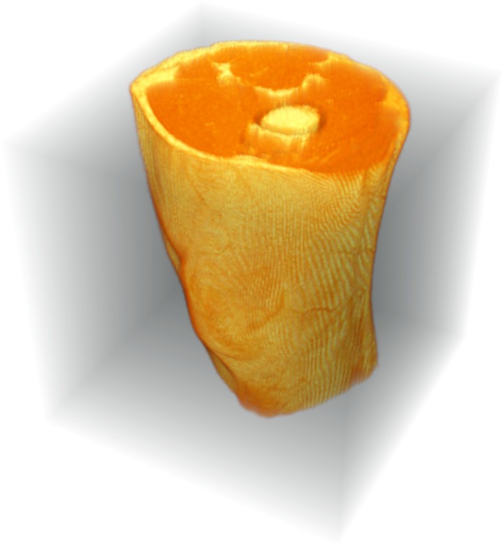
The underlying data consists of the measured density values at each voxel position, meaning this array has a shape of:
M = ⟨D,H,W⟩ -> ℝ
The axes of this array are:
| axis | name | meaning | part space |
|---|---|---|---|
| 1 | Z |
lateral position of a voxel | 1..D |
| 2 | Y |
vertical position of a voxel | 1..H |
| 3 | X |
horizontal position of a voxel | 1..W |
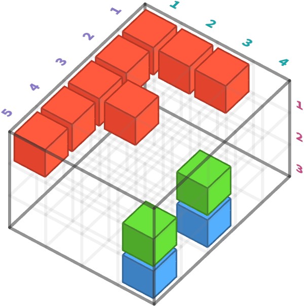
As a toy example, consider this 3-array of shape ⟨3,3,3⟩ representing a small shape:
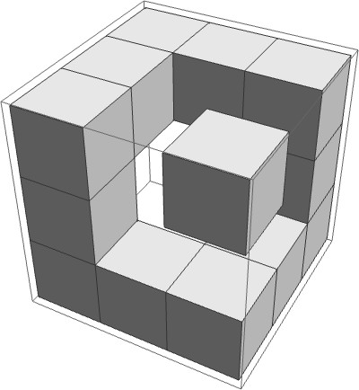
Here is the corresponding 3-array:
    ⎡⎡[1 1 1 ⎡[0 0 1 ⎡[0 0 1
M = ⎢⎢[1 0 0 ⎢[0 0 0 ⎢[0 0 1
    ⎣⎣[1 0 1 ⎣[1 0 0 ⎣[1 1 1
Vector fields #
Consider a so-called vector field which describes the direction and speed that the wind is blowing over some regular grid of locations on the earth. We might have obtained this by making actual measurements using devices likes anemometers. Or, more likely, we could have run a computer simulation that is constructing a prediction of how wind will behave in some future scenario, and we have taken data from this simulation at a particular time point.
Let’s see a stylized picture of what such a vector field might look like, which we might imagine is depicting the “eye of a hurricane”. We’ve labeled the frame to indicate the latitude and longitude of the grid points relative to some reference point.
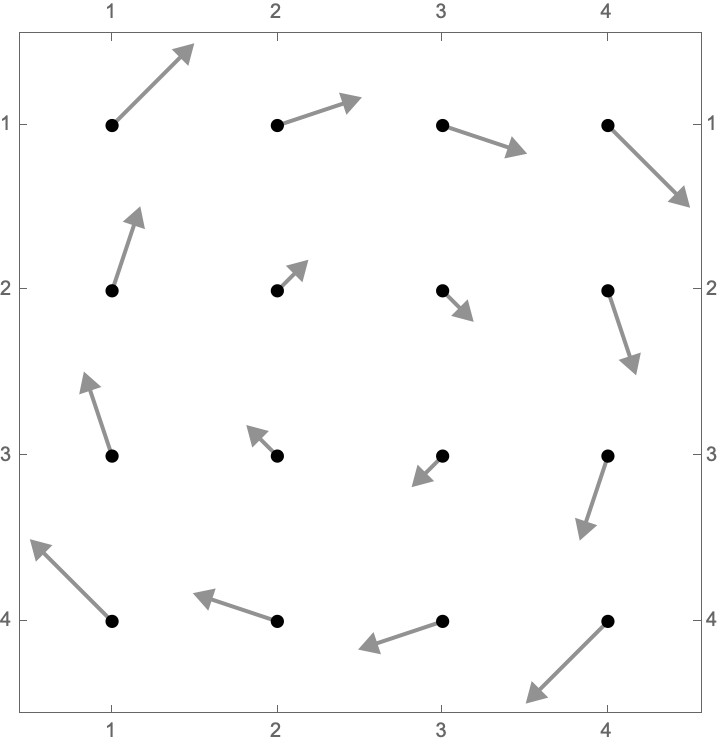
Each of the arrows in the plot above depicts a wind vector, a combination of a velocity and direction that the wind is blowing. Here we show two of these wind vectors and their corresponding representation in terms of the x and y components:
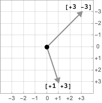
What is the data required to represent the entire wind vector field? A grid point is described by a latitude and longitude, so our key will need at least two parts. The third part of our key will pick either the x or y component of the wind vector. The value at that cell is then a real number which describes the component of the wind vector in that direction:
| axis | meaning | part space |
|---|---|---|
1 |
longitude of a grid point | 1..4 |
2 |
lattitude of a grid point | 1..4 |
3 |
component of the wind vector | {x,y} |
Hence the entire wind vector field is represented by a 3-array:
W : ⟨4,4,2⟩ -> ℝ
The actual data underlying this vector field for our hurricane is shown below:
    ⎡[[-3 +3 [-1 +3 [+1 +3 [+3 +3
W = ⎢[[-3 +1 [-1 +1 [+1 +1 [+3 +1
    ⎢[[-3 -1 [-1 -1 [+1 -1 [+3 -1
    ⎣[[-3 -3 [-1 -3 [+1 -3 [+3 -3
For example, the [+3 +3 at the top right of the matrix indicates that the wind blows down and to the right at that gridpoint.
Graphs #
As a quite different kind of example, we can also represent graphs or networks via their adjacency. Recall that a graph consists of a set V of vertices and a collection of edges that connect these vertices. Here’s a simple example of a directed graph with vertices V = a..e = {a,b,c,d,e}:
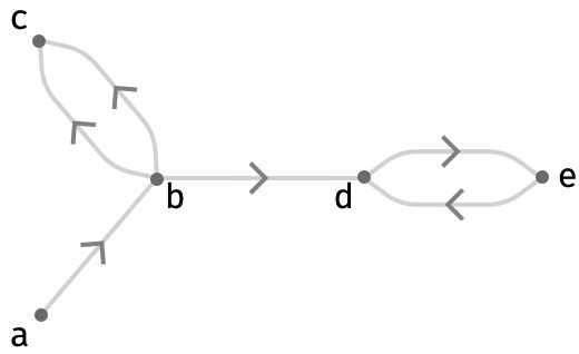
Each edge is described by a source vertex and a target vertex. To describe an edge therefore we need two axes:
| axis | meaning | part space |
|---|---|---|
1 |
source vertex of edge | V |
2 |
target vertex of edge | V |
A cell A[s,t] in the matrix will contain the number of edges of the form s |-> t in the graph. Therefore the adjacency information is described as an adjacency matrix of type:
A : ⟨V,V⟩ -> ℕ
For the graph above, we have the corresponding adjacency matrix:
        a b c d e
    a ⎡[0 1 0 0 0
    b ⎢[0 0 2 1 0
A = c ⎢[0 0 0 0 0
    d ⎢[0 0 0 0 1
    e ⎣[0 0 0 1 0
Hypergraphs #
A hypergraph is similar to a graph, but allows the edges to involve a variable number of vertices.
Consider the following ordered 3-graph, which is a hypergraph in which each edge is composed of 3 vertices rather than 2. The vertices are the integers 1..4:
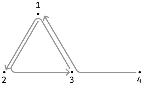
Each hyperedge is described by a source vertex, a middle vertex, and a target vertex. To describe a hyperedge therefore we need three axes:
| axis | meaning | part space |
|---|---|---|
1 |
source vertex of hyperedge | V |
2 |
middle vertex of hyperedge | V |
3 |
target vertex of hyperedge | V |
A cell A[s,m,t] in the matrix will contain the number of hyperedges of the form s |-m-> t in the graph. Therefore the adjacency information is described as an adjacency 3-array of type:
A : ⟨V,V,V⟩ -> ℕ
The hypergraph above is described by the following adjacency 3-array:
    ⎡⎡[0 0 0 0 ⎡[0 0 0 0 ⎡[0 1 0 0 ⎡[0 0 0 0
A = ⎢⎢[0 0 1 0 ⎢[0 0 0 0 ⎢[0 0 0 0 ⎢[0 0 0 0
    ⎢⎢[0 0 0 0 ⎢[0 0 0 0 ⎢[0 0 0 0 ⎢[1 0 0 0
    ⎣⎣[0 0 0 0 ⎣[0 0 0 0 ⎣[0 0 0 0 ⎣[0 0 0 0
To interpret this array, notice that the non-zero entries are at ⟨1,2,3⟩, ⟨3,1,2⟩, and ⟨4,3,1⟩, which correspond to the source, middle, and target of the three hyperedges shown above.
Primitive operations #
Introduction #
Underlying the vast majority of array programming lie a handful of primitive operations that can derive these more complex computations and that have a particularly simple form. Some of these operate on single arrays, others on multiple arrays. Some of these are parameterized by one or more integers giving the axes they operate on.
Here we list the operations we will discuss, their number of inputs (#), along with a brief description of what they accomplish:
| name | # | description | example |
|---|---|---|---|
| lift | n | apply fn to matching cells | A +↑ B |
| aggregate | 1 | use a fn to summarize an axis | sum2(A) |
| merge | 1 | merge multiple parts of an axis together | sumR2(A) |
| broadcast | 1 | introduce constant novel axis | A2➜ |
| transpose | 1 | permute the order of the axes | Aσ |
| nest unnest |
1 | turn an array into nested arrays turn nested arrays into one array |
A2≻ |
| diagonal | 1 | obtain a diagonal along an array | M1:(1,2) |
| pick | 2 | pick cells by their keys | A[P] |
This list isn’t exhaustive! You won’t see familiar operations like finding the sort order of a vector, or the positions of minimum and maximum values. Not that these operations aren’t important, but they do end up entraining some details that I don’t think add much to the larger framework.
Cellwise definitions #
In array programming, we often compute an array (the “output array”) that depends on other arrays ("input arrays"). To do this, we work backwards, defining how to derive each output cell from input cells.
Here are some examples of these kinds of cellwise definitions:
 M[i,j] ≡ V[i] + W[j]
 M[i,j] ≡ S[]
   V[i] ≡ V[i] * M[i]
    S[] ≡ sumi∈1..N{ V[i] }
In English, the first definition says: to compute the value of the cell of M at key (i,j) , add the cell of V at key (i) and the cell of W at key (j). Here i,j stand in for any valid part of the corresponding part spaces.
Cellwise definitions are the most flexible kind of definition (depending on what operations we allow on the right hand side), but can often be decomposed into other, primitive operations. We’ll shortly elaborate on a set of primitive operations that encompass most of what array programming is about.
Colourful notation #
In cellwise definitions, we can use symbols to indicate parts that can vary over any value allowed by the shapes of the corresponding arrays:
P[i,j] ≡ A[i] + B[j]
To make it easier to see that i and j occur in two places in the cellwise definition, let us colour them:
P[i,j] ≡ A[i] + B[j]
We’ll always choose the colours to match the colours of nested brackets when we give concrete examples, which makes things particularly easy to follow, e.g.:
⎡[1 2   ⎡1
⎢[3 4 = ⎢3 + [0 1
⎣[5 6   ⎣5
We can go further, however, and only use coloured disks to represent parts, replacing the use of roman symbols for that role:
P[●,●] ≡ A[●] + B[●]
We’ll also often simultaneously use a coloured square to represent the size of an axis in a shape, like so:
P : ⟨■,■⟩
A : ⟨■⟩
B : ⟨■⟩

P[●,●] ≡ A[●] + B[●]
Here, the ■ in ⟨■,■⟩ represents a symbolic size that we leave unspecified, whereas the ● in A[●] represents a symbolic part that is taken from the corresponding part space 1..■. This is the equivalent definition spelled out with symbols:
P : ⟨m,n⟩
A : ⟨m⟩
B : ⟨n⟩

P[i,j] ≡ A[i] + B[j]
Lift op #
In some sense the simplest of the operations, lifted operations are expressed by lifting an n-ary operation f on the underlying value space of several arrays into n-ary operations on the arrays themselves. This operation is not required to be commutative, associative, etc., although the lifted version of the operation will inherit these properties (suitably defined) if they exist.
Lifted operations are also referred to as elementwise operations in array programming.
The definition of an lifted operation is extremely simple. For arbitrary n-ary function
f : Vn -> V
the lifted operation (written f↑) operates on arrays with identical key spaces K:
f↑ : (K->V)n -> (K->V)
The cellwise definition is:
 f(A,B,…) : ⟨■,■,■,…⟩ -> V
f↑(A,B,…) : ⟨■,■,■,…⟩ -> V

f↑(A,B,…)[●,●,●,…] = f(A[●,●,●,…], B[●,●,●,…], …)
Put simple, we feed the provided key to each of the input arrays and then pass the corresponding values to f.
Array circuit #
We can depict this situation graphically using an array circuit, a diagram in which arrays (functions) are boxes and keys and values are purple and gray wires respectively. Computation occurs as we go down the page.
The entire outer box is the array we are defining (here, being f↑(A,B,C)), and the boxes in the interior show how parts of the key are used to look up values of individual vectors A,B,C to compute a value for the entire lifted array:
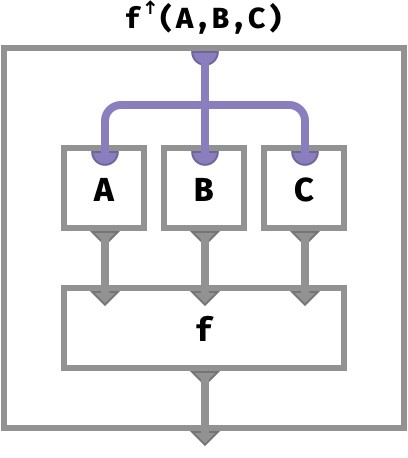
We will see many more examples of these diagrams in the coming sections.
Examples #
Adding two 3-vectors of integers:
(A +↑ B)[●] ≡ A[●] + B[●]

    ⎡1       ⎡0            ⎡1
A = ⎢2   B = ⎢3   A +↑ B = ⎢5
    ⎣3       ⎣5            ⎣8
Taking the logical and (∧) of two ⟨2,2⟩ matrices of boolean values:
(A ∧↑ B)[●,●] ≡ A[●,●] ∧ B[●,●]

A = ⎡[F T   B = ⎡[F F   A ∧↑ B = ⎡[F F
    ⎣[F T       ⎣[T T            ⎣[F T
Negating a 3-array of booleans:
(¬↑A)[●,●,●] ≡ ¬(A[●,●,●])

A = ⎡⎡[T T F   ¬↑A = ⎡⎡[F F T
    ⎢⎣[T F F         ⎢⎣[F T T
    ⎢⎡[F T F         ⎢⎡[T F T
    ⎣⎣[T F F         ⎣⎣[F T T
Algebra #
If you are familiar with some common algebraic structures, this table is a summary of the kinds of operations that are typically lifted:
| value space | algebraic structure | operations that can be lifted |
|---|---|---|
ℝ |
field | addition (+), multiplication (*)subtraction ( -), division (/)negation ( -□), inverse (□ -1) |
ℕ, ℝ, ℤ |
semiring | addition (+), multiplication (*) |
B |
semiring | and (∧), or (∨), xor (⊻), not (¬) |
P(X) |
lattice | meet (∧), join (∨) |
Technicalities #
For simplicity, we presented an lifted function f:Vn -> V as an n-argument function that takes arguments in V and produces a result in V. This is actually unnecessary, we can consider a more general kind of function that takes arguments in any mixture of value spaces, and produces an output in any value space at all:
f : (V1,V2,...,Vn) -> W
The lifted function the operates on arrays with some shared key space K and the corresponding value spaces Vi:
f↑ : (K->V1, K->V2,..., K->Vn) -> (K->W)
An example of this would occur if we wish to divide a vector of integers by a vector of positive natural numbers to obtain a vector of rational numbers. The underlying function here is defined by:
div : (ℤ, ℕ+) -> ℚ
div(r, n) ≡ r / n
This lifts to an array operation div↑ : (⟨…⟩->ℤ, ⟨…⟩->ℕ+) -> (⟨…⟩->ℚ):
    ⎛⎡1  ⎡3⎞   ⎡1/3
div↑⎜⎢2, ⎢2⎟ = ⎢1
    ⎝⎣3  ⎣1⎠   ⎣3
Aggregate op #
When we aggregate an array, we effectively remove an axis by taking all cells along that axis and “summarizing” them.
This summary is achieved by a commutative n-ary aggregator function agg that applies to the value space. Commutativity is required to ensure that it does not matter what order we provide the values to this aggregator, since there may not be a natural order to parts in a part space.
An aggregator can be seen as a function that takes a multiset (or bag) of V to a single V:
agg : V* -> V
Some common examples of value spaces and typical aggregations are given below:
| value space | algebraic structure | aggregations | example |
|---|---|---|---|
ℝ |
field | mean | mean{ 1, 2 } = 1.5 |
ℕ, ℝ, ℤ |
semiring | sum, product, max, min | sum{ 1, 2, 3 } = 6 |
B |
semiring | and (∧), or (∨), xor (⊻) |
or{ F, T } = T |
Notationally, we can write aggn(A) to indicate we are aggregating over the n‘th axis of A using the aggregator agg. The abstract cellwise definition is as follows:
     A  : ⟨…,■n,…⟩ -> V
aggn(A) : ⟨…⟩ -> V

aggn(A)[…] = agg{ A[…,●n,…] | ●n ∈ ■n }
Here are some examples of such aggregations on arrays of different arity, with cellwise definitions and corresponding examples.
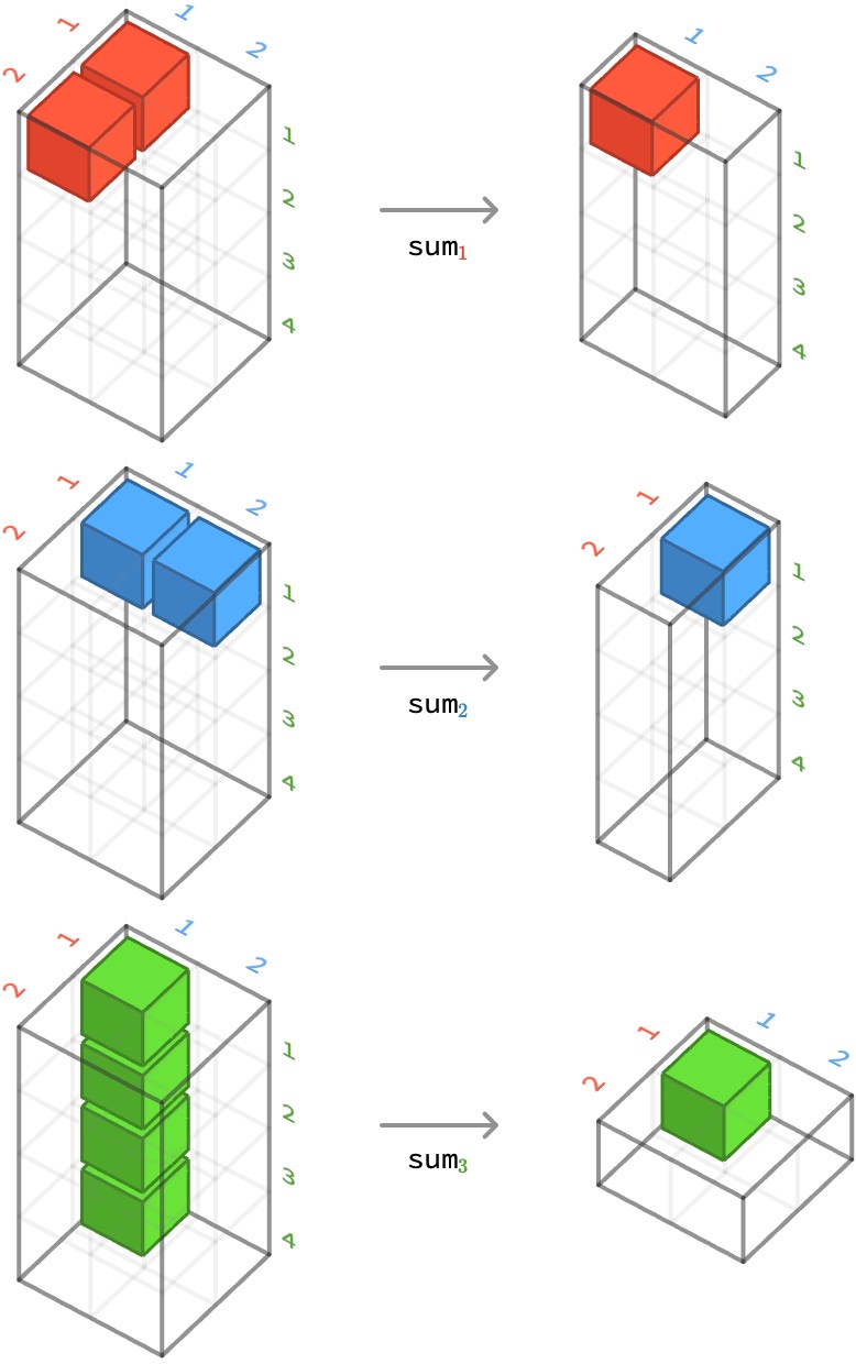
Summing a 3-array #
First, let’s considering summing over the second axis of a ⟨2,2,4⟩-array:
sum2(H)[●,●] ≡ sum●∈1..2{ H[●,●,●] } = H[●,1,●] + H[●,2,●]

sum2 ⎡⎡[1 1 0 2 = ⎡ [1 1 0 2
     ⎢⎣[0 0 0 0   ⎣ [2 1 3 2
     ⎢⎡[2 1 1 0
     ⎣⎣[0 0 2 2
To illustrate how this works more vividly, let’s show the result of aggregating each axis in turn. For each example, we highlight how a particular cell of the output aggregates several cells from the input:
sum1 ⎡⎡[1 1 0 2 =  ⎡[3 2 1 2
     ⎢⎣[0 0 0 0    ⎣[0 0 2 2
     ⎢⎡[2 1 1 0
     ⎣⎣[0 0 2 2

sum2 ⎡⎡[1 1 0 2 = ⎡ [1 1 0 2
     ⎢⎣[0 0 0 0   ⎣ [2 1 3 2
     ⎢⎡[2 1 1 0
     ⎣⎣[0 0 2 2

sum3 ⎡⎡[1 1 0 2 = ⎡⎡ 4
     ⎢⎣[0 0 0 0   ⎢⎣ 0
     ⎢⎡[2 1 1 0   ⎢⎡ 4
     ⎣⎣[0 0 2 2   ⎣⎣ 4
We can also present this cubically, by depicting how a cell of the output of the aggregation depends on a set of cells of the input array:
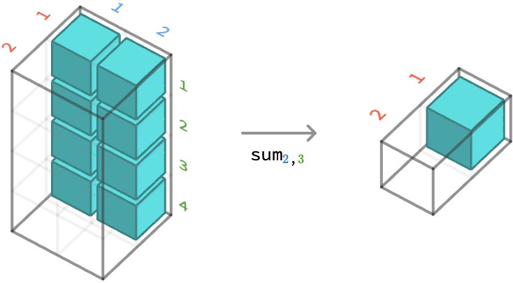
Multiple axes #
We can also aggregate multiple axes simultaneously. Here we show multi-aggregation over axes 2 and 3 on the same array:
sum2,3 ⎡⎡[1 1 0 2 = ⎡ 4
       ⎢⎣[0 0 0 0   ⎢
       ⎢⎡[2 1 1 0   ⎢
       ⎣⎣[0 0 2 2   ⎣ 8
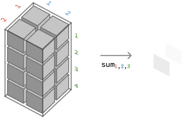
Another important case is aggregating over all axes:
sum1,2,3 ⎡⎡[1 1 0 2 = 12
        ⎢⎣[0 0 0 0
        ⎢⎡[2 1 1 0
        ⎣⎣[0 0 2 2
Maximum over a matrix #
Next, let’s considering taking the maximum over the first axis of a ⟨2,4⟩-matrix:
max1(M)[●] ≡ max●∈1..2{ M[●,●] } = max(M[1,●], M[2,●])

max1 ⎡[2 1 1 0 = [2 1 2 3
     ⎣[0 0 2 3
And over the second axis:
max2(M)[●] ≡ max●∈1..4{ M[●,●] } = max(M[●,1], M[●,2], M[●,3], M[●,4])

max2 ⎡[2 1 1 0 = ⎡2
     ⎣[0 0 2 3   ⎣3
Logical ∧ over a vector #
Lastly, let’s aggregate logical and over the sole axis of 3-vector of boolean values:
and1(V)[] ≡ and●∈1..3{ V[●] } = V[1] ∧ V[2] ∧ V[3]

and1 [T F F] = F
Technicalities #
The aggregator agg need not produce a value in V. In fact, it may produce a value in any value space W:
    agg : V* -> W
     A  : ⟨…,■n,…⟩ -> V
aggn(A) : ⟨…⟩ -> W
Array circuit #
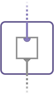
We can depict an aggregation of the second axis of matrix M as follows.
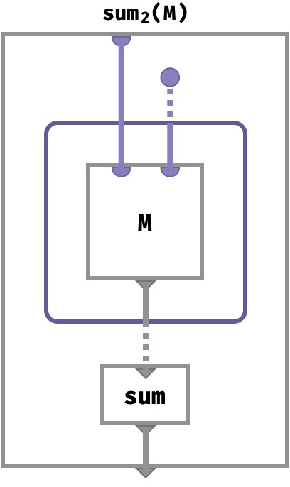
Multiset subcircuits #
We just introduced the following circuit to compute summing over the columns of a matrix:
But what does this circuit actually mean?
Dotted wires indicate multiset wires: these carry not individual parts (or values) but entire multisets of parts (or values). A multiset is also called a bag or orderless list. It’s like a set that can contain individual elements more than once.
This particular circuit fragment has a solid purple disk: this stands for a relation that outputs an entire part space – in this case the column indices for our matrix M. It emits a dotted wire, representing a wire carrying a multiset that contains every element of this part space exactly once:
The inner shaded purple box “maps” over multisets: it computes an output (a setting for the solid gray wire) for every individual value in the multiset wire that enters it, using ordinary circuit semantics for the subcircuit it encloses. It collects these outputs, one for each setting of the input multiset, and these are outputs form another multiset that leaves on the dotted gray output wire:
This notation is the circuit incarnation of a familiar idea in mathematics called a set comprehension, typically written { ⋯ | ⋯ }. More precisely it is a multiset comprehension, since we are constructing a multiset rather than a set. Let’s go back to our original diagram:
We think of this as feeding the first part of the matrix key with a single value x ∈ X from the first part space (the solid purple line), and feeding the second part of the matrix key with an entire multiset Y ∈ Y* worth of parts (the dashed purple line):
x : X
Y : Y*
Y = mset{ y | y ∈ Y }
We wrote mset{ ⋯ } rather than { ⋯ } to distinguish this multiset comprehension from ordinary set comprehension notation .
After being threaded over the array V, this multiset of inputs x results in an entire multiset z of output cell values, also indicated with a dashed gray line.
z : V*
z = mset{ M[x,y] | y ∈ Y }
Finally, we apply the aggregation function sum : V* -> V to this multiset to obtain a single value v ∈ V:
v : V
v = sum( z )
  = sum( mset{ M[x,y] | y ∈ Y } )
  = sum{ M[x,y] | y ∈ Y }
Multiset syntactic sugar #
To avoid compex diagrams arising from aggregations, we will resort to a natural form of syntactic sugar that pulls the dashed multiset wires into the multiset constructor box, or even into the array itself (if only a single named array is involved). The aggregation function to apply to the output is then written at the bottom of the box, next to the output wire. Here’s the sugar:
Sweet!
Merge op #
Very similar to aggregation is merging. Merging can be seen as a kind of aggregation that does not destroy an axis, but merely changes its part space.
Some practical examples of merging are:
-
downsampling or upsampling an image to have different dimensions
-
making the bins of a histogram coarser by summing together several cells
Like aggregation, merging is performed via a particular aggregation function applied against an axis, except it also involves a relation R that determines how the part space of the relevant axis will be changed. We write a merging operation on an array A as aggRn:
  R ⊂ ■ × ■
agg : V* -> V

      A  : ⟨…,■n,…⟩ -> V
aggRn(A) : ⟨…,■n,…⟩ -> V
The relation R determines which cells of A are aggregated to form cells of the resulting array, via this cellwise definition:
aggRn(A)[…,●n,…] ≡ agg{ A[…,●n,…] | R(●,●) }
In other words, we aggregate together into a given part ● of the output all those cells of the input with part ● that are R-related to it. The motivation for using a relation rather than a function is that it gives us the freedom to either ignore the contents of a cell, use it precisely once, or use it in multiple cells of the binned result.
Let’s look at some examples using a 3-vector V:⟨■⟩ with part space ■={a,b,c}.
We will merge this to a 2-vector W:⟨■⟩ with part space ■={x,y}.
     a b c
V = [1 2 3]

W = sumR1(V)
We will now show the computation of W for several choices of relation R:■×■:
                          x y
R = {}               W = [0 0
R = {a↦x}            W = [1 0
R = {a↦x,b↦x}        W = [3 0
R = {a↦x,a↦y}        W = [1 1
R = {a↦x,b↦y,c↦y}    W = [1 5
We can think of the relation as “pushing” cells of the input array V into cells of the output array W, with the aggregation operation determining how multiple input cells will be combined when they are all pushed to the same output cell.
Applications #
Let’s revisit our histogram of passenger ages on the titanic. Recall it looked like this:
H = [51 31 25 118 183 161 130 102 69 66 43 27 27 5 6
Let us now merge several of these bins together to form a coarser histogram H'. The number of counts should be summed, of course. We will add groups of 3 bins at a time, dropping the final bin of 70-74. Here we visualize the relation R and how it maps parts of H to parts of H':
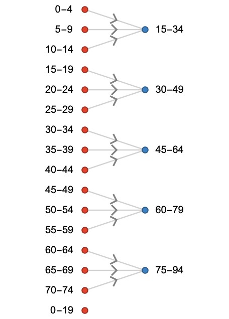
The result of merging is given by:
H' = sumR1(H) = [107 462 301 136 38
Array circuit #
We can depict the merging of a vector V along its only axis as the following circuit:
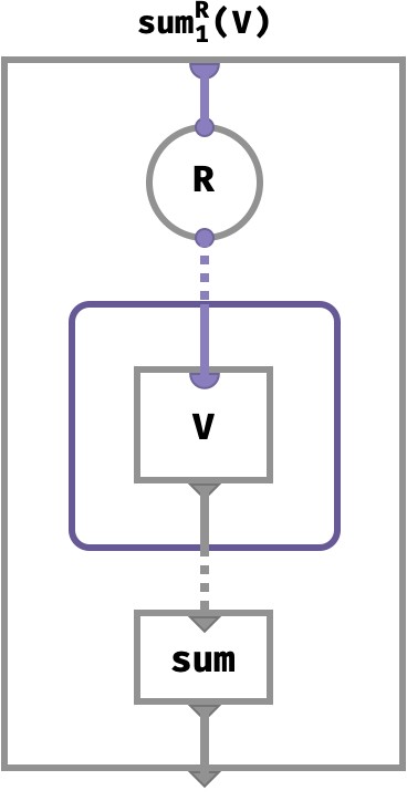
Here, the relation R takes an ordinary part input x ∈ X and yields an entire multiset Y ∈ Y* worth of parts (the dashed purple line) that corresponds to all elements in Y that are R-related to x:
x : X
Y : Y*

Y = mset{ y | R(x,y), y ∈ Y }
This results in an entire multiset z of output cell values, also indicated with a dashed gray line.
z : V*
z = mset{ M[x,y] | R(x,y), y ∈ Y }
Finally, we apply the aggregation function sum : V* -> V to this multiset to obtain a single value v ∈ V:
v = sum( z )
  = sum( mset{ M[x,y] | R(x,y), y ∈ Y } )
  = sum{ M[x,y] | R(x,y), y ∈ Y }
Broadcast op #
Broadcasting repeats the cell of an array across additional, novel axis that it didn’t have before. As an orienting example, consider repeating the cells of a vector so that it becomes a matrix:
⎡1     ⎡[1 1
⎢2 |-> ⎢[2 2
⎣3     ⎣[3 3
Cellwise, this corresponds to ignoring the parts of keys corresponding to the novel axis. In the case above, we can write this cellwise as saying that the column of the matrix M isn’t important, only the row of the matrix determines the value of the cell, which is derived from the value of the vector V:
M[r,c] ≡ V[r]
Here we give some other examples of cellwise definitions, showing how there are often multiple ways we do this kind of operation:
| z | z |
|---|---|
| broadcast scalar to vector | V[i] ≡ S[] |
| broadcast vector to matrix | M[r,c] ≡ V[r] |
| broadcast scalar to matrix | M[r,c] ≡ S[] |
| broadcast matrix to 3-array | H[i,j,k] ≡ M[i,j] |
We will denote broadcasting by Aa➜s, where a is the position in axis list where an axis of size s will be inserted. If A is an n-array, the position a can range from 1 to n+1.
Let’s look at some examples of how broadcasting affects the shape of an input 3-array A:⟨1,2,3⟩:
| z | z |
|---|---|
A1->9 |
⟨9,1,2,3⟩ |
A2->9 |
⟨1,9,2,3⟩ |
A3->9 |
⟨1,2,9,3⟩ |
A4->9 |
⟨1,2,3,9⟩ |
Here are concrete examples of broadcasting a vector U = [1 2 3]:
U1->2 = ⎡[1 2 3
       ⎣[1 2 3

U2->3 = ⎡[1 1 1
       ⎢[2 2 2
       ⎣[3 3 3
Broadcasting a scalar S = 9:
    S1->2 = [9 9

S1->2,2->3 = ⎡[9 9 9
           ⎣[9 9 9
In the functional perspective, the broadcasted array An➜s takes one additional argument over A, but drops it and then passes the rest to A. Here is the general cellwise definition of broadcasting:
   A:⟨…⟩ -> V
An➜s:⟨…,sn,…⟩ -> V

An➜s[…,●n,…] ≡ A[…]
Here, we use the ellipsis … to indicate the arguments except the one explicitly indexed. When appearing on the right hand side, the … refers to the combination of all the ellipses on the left.
This behavior of dropping a part from the key tuple explains why broadcasting produces an array that is “constant” across a particular axis: if we hold all other parts the same, and vary the part of a broadcasted axis, the cell value will not change, since it does not depend on this particular part.
Combination with lift #
We can use lifted operations in conjunction with broadcasting to allow us to combine arrays that have dissimilar shapes.
For example, take the matrix M:⟨3,2⟩ and the vector V:⟨3⟩:
    ⎡[1 0       ⎡1
M = ⎢[0 1   V = ⎢2
    ⎣[1 1       ⎣3
We’ve displayed the 3-vector in column form, but this is just to suggest that we wish to multiply each cell of V with the corresponding row of M. In other words, we want:
M'[r,c] ≡ V[r] * M[r,c]

        ⎡[1 0
M'     = ⎢[0 2
        ⎣[3 3
However, because M and V have different shapes, they cannot be simply lift-multiplied. We can however broadcast V as follows:
        ⎡[1 1
V2->2  = ⎢[2 2
        ⎣[3 3
We now have two matrices of the same shape that can be lift-multiplied:
            ⎡[1 0    ⎡[1 1   ⎡[1 0
M *↑ V2->2 = ⎢[0 1 *↑ ⎢[2 2 = ⎢[0 2 = M'
            ⎣[1 1    ⎣[3 3   ⎣[3 3
When performing broadcasting followed by lifted operations in this way, we need not specify the size of the novel axis, since it is implied by the shape of the other arrays participating in the lifted operation. Hence we can just write M *↑ V2->.
Array circuit #
We can depict a broadcasting of a vector V to a matrix along the first and second axis respectively as the circuits:
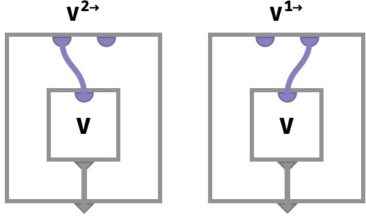
Notice the second part of the key space is simply ignored. Only the first part is fed to the vector V to obtain a value.
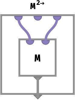
Here we show the broadcasting of a matrix M to a 3-array by introducing a novel axis at the second position:
Deriving familiar operations #
We’re now in a position to derive some of the array operations that might familiar from linear algebra.
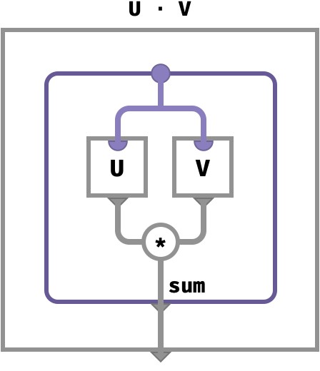
Dot product #
The traditional definition of vector dot product U ⋅ V is given cellwise below. We show how to express this in terms of primitive operations.
    U : ⟨■⟩
    V : ⟨■⟩
U ⋅ V : ⟨⟩

(U ⋅ V)[] ≡ sum●∈■{ U[●] * V[●] }
Here’s how we can achieve this computation in terms of primitive lifted and aggregation ops:
(U ⋅ V)[] ≡ sum●∈■{  U[●] * V[●] }    given
          = sum●∈■{  (U *↑ V)[●] }    def of lifted *
          = sum1( U *↑ V )[●]         def of aggregate sum
          ∴
 U ⋅ V    ≡ sum1( U *↑ V )
Let’s illustrate this as a circuit diagram, using the aggregation circuit sugar we introduced earlier:
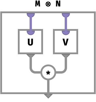
Tensor product #
The tensor product of two vectors is a matrix defined cellwise as follows:
    U : ⟨■⟩
    V : ⟨■⟩
U ⊗ V : ⟨■,■⟩


(U ⊗ V)[●,●] ≡ U[●] * V[●]
We must use broadcast to express this in terms of primitive operations:
(U ⊗ V)[●,●] ≡   U[●  ]  *   V[  ●]    given
             = U2➜[●,●] *↑ V1➜[●,●]    def of broadcast
             =    (U2➜ *↑ V1➜)[●,●]    def of lifted *
             ∴
 U ⊗ V       ≡ U2➜ * V1➜
The circuit for this is:
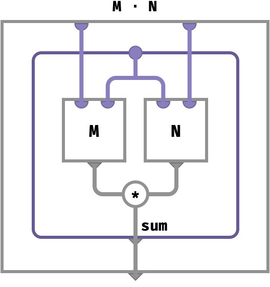
Matrix multiplication #
Using the traditional definition of matrix multiplication M ⋅ N, we have the following cellwise description:
    M : ⟨■,■⟩
    N : ⟨■,■⟩
M ⋅ N : ⟨■,■⟩


(M ⋅ N)[●,●] = ∑●∈■ M[●,●] * N[●,●]
To compute this with our primitive ops, we need not only broadcasting and lifted operations but aggregation as well:
(M ⋅ N)[●,●] ≡ sum●∈■{   M[●,●  ] *   N[  ●,●] }   def of ⋅
             = sum●∈■{ M3➜[●,●,●] * 1➜N[●,●,●] }   def of broadcast
             = sum●∈■{      (M3➜ *↑ 1➜N)[●,●,●] }   def of lifted *
             =          sum2(M3➜ *↑ 1➜N)[●,  ●]     def of aggregate sum
             ∴
 M ⋅ N       ≡ sum2(M3➜ * 1➜N)
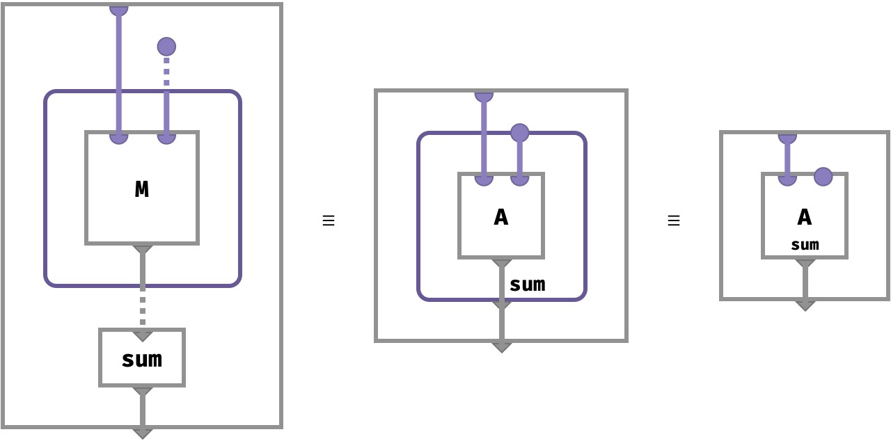
The circuit diagram for this is a sort of hybrid of the previous two:
The diagrammatic sugar hid the role of multisets from us. Let’s have our tea without sugar to see the computation more explicitly:
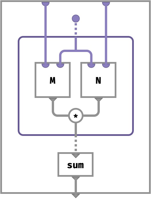
Here, dotted lines carry multisets of values, originating in the part space for the second axis of M / first axis of N. When the inner purple frame is penetrated, these multiset key wires take on particular concrete values. The single output value then becomes a multiset of values that correspond to the multiset of outputs. This multiplicity is finally discharged by the sum aggregation function. The inner gray bubble represents an ordinary computation that is repeated for every part in the multiset of parts that enters it.
Transpose op #
Transpose re-arranges the order of axes, but leaves the contents of cells otherwise unaffected.
The most familiar instance of transpose is the transpose of a matrix, which interchanges rows and columns:
Mᵀ[r,c] ≡ M[c,r]
Harking back to the section on image arrays, we can also convert between the YXC and CYX conventions:
I'[y,x,c] ≡ I[c,y,x]
The most general kind of transpose applies a permutation σ of the integers 1..n, which we notate as Aσ:
Aσ[●1,●2,…,●n] ≡ A[●σ(1),●σ(2),…,●σ(n)]
If we recall that A[●1,●2,…,●n] is shorthand for A( (●1,●2,…,●n) ), we can see that σ acts by permuting the components of the key:
(●1,●2,…,●n) |-> (●σ(1),●σ(2),…,●σ(n))
Applications #
Matrix transpose and image conversion can then be written using cycle notation, in which we write (a,b,c) to mean the permutation {a↦b,b↦c,c↦a}:
Mᵀ = M(1,2)
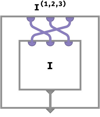
I' = I(1,2,3)
Array circuit #
Matrix transpose M(1,2) has the following array circuit:
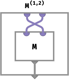
Notice that the wires corresponding to the first and second parts of the key space are swapped before being plugged in to M.
The circuit for the 3-array transpose I(1,2,3) is shown below:
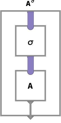
In the general case we have an arbitrary permutation σ that re-arranges the order of n wires before applying an array A. Here, the thick purple wires stand for an arbitrary “bundle” of n wires:
Nest op #
In the functional perspective, we see an array A as a function A:K->V, where K is the key space and V is the value space.
For example, an integer-valued matrix M of shape ⟨3,2⟩ is merely a function M:⟨3,2⟩ -> ℤ.
Let’s work with the example matrix M = [ [1 2] [3 4] [5 6] ], which can be seen a vector-of-vectors in two distinct ways.
The first way is as a 3-vector whose cells are 2-vectors, in other words a function A:⟨3⟩->⟨2⟩->ℤ:
⎡x⎤           x = [1 2]
⎢y⎥   where   y = [3 4]
⎣z⎦           z = [5 6]
The second way is as a 2-vector whose cells are 3-vectors, in other words a function A:⟨2⟩->⟨3⟩->ℤ:
                    ⎡1⎤       ⎡2⎤
[a b]   where   a = ⎢3⎥   b = ⎢4⎥
                    ⎣5⎦       ⎣6⎦
In computer science, the isomorphism between functions of type A⨉B->C and A->B->C is known as currying. We will be currying the n‘th argument of a function to yield a function taking \(n\mathbin{ - }1\) arguments and returning a function of one argument.
We will denote the nesting the n‘th axis of A with An≻, which has the following cellwise definition:
An≻[…][●] ≡ A[…,●n,…]
This simply injects the part ● into the key tuple at position n.
Nesting the n‘th axis moves that axis into the value space, meaning the nesting’s cells are vectors. Here is how we can state that type-wise:
   A:⟨…,■n,…⟩ -> V
 An≻:⟨…⟩ -> ⟨■⟩ -> V
We can now write the two ways of nesting the example matrix M:⟨3,2⟩:
    ⎡[1 2
M = ⎢[3 4
    ⎣[5 6
Nesting on the first axis is defined by:
M1≻[●][●] ≡ M[●,●]
Computing the two cells of this vector-of-vectors gives us the two column vectors of M:
M1≻[1] = M[●,1] = [1 3 5]
M1≻[2] = M[●,2] = [2 4 6]
Nesting on the second axis is defined by:
M2≻[●][●] ≡ M[●,●]
Computing the three cells of this vector-of-vectors gives us the three row vectors of M:
M2≻[1] = M[1,●] = [1 2]
M2≻[2] = M[2,●] = [3 4]
M2≻[3] = M[3,●] = [5 6]
Multiple axes #
Nesting multiple axes simultaneously make the cells of the nested array into arbitrary arrays. For example:
A1,3≻[●][●,●] ≡ A[●,●,●]
Correspondence with nested notation #
Note that the way we write arrays an array of type ⟨■,■,■,…⟩ -> V is naturally identical with the way we would write an array of shape ⟨■⟩->⟨■⟩->⟨■⟩-> … ->V.
To see this, let’s take the array H : ⟨2,2,4⟩ -> ℤ defined below:
⎡⎡[1 1 0 2
⎢⎣[0 0 0 0
⎢⎡[2 1 1 0
⎣⎣[0 0 2 2
Let’s visually group cells that align along the third axis:
⎡⎡ ([1 1 0 2
⎢⎣ ([0 0 0 0
⎢⎡ ([2 1 1 0
⎣⎣ ([0 0 2 2
We can see that each of these is itself a vector with a single axis. Therefore, our notation makes visual the bijection between a 3-array and an ordinary matrix whose cells contain vectors:
H : ⟨2,2,4⟩ -> ℤ <==> H3≻ : ⟨2,2⟩ -> ⟨4⟩ -> ℤ
Similarly, let’s visually group cells that align along the second axis:
⎡ ⎛⎡[1 1 0 2
⎢ ⎝⎣[0 0 0 0
⎢
⎢ ⎛⎡[2 1 1 0
⎣ ⎝⎣[0 0 2 2
This time, we see that our notation makes visual the bijection between a 3-array and an ordinary vector whose cells contain matrices:
H : ⟨2,2,4⟩ -> ℤ <==> H2,3≻ : ⟨2⟩ -> ⟨2,4⟩ -> ℤ
Lastly, we have the somewhat subtle fact that a 3-array can be seen as a scalar array whose only cell happens to contain a 3-array:
⎛⎡⎡[1 1 0 2
⎜⎢⎣[0 0 0 0
⎜⎢⎡[2 1 1 0
⎝⎣⎣[0 0 2 2
This is the bijection:
H : ⟨2,2,4⟩ -> ℤ <==> H1,2,3≻ : ⟨⟩ -> ⟨2,2,4⟩ -> ℤ
This animates a somewhat philosophical question: is a matrix different from a vector of vectors? In array algebra, the answer is ‘yes’, but nesting and unnesting gives us a canonical way to see an n-array as a Matroska doll of vectors that contain vectors that contain … (n times).
Applications #
Returning to our original example of a colour image array I : ⟨H,W,3⟩ -> ℝ, we pointed out earlier that we can see the colour channel axis as describing a single pixel.
Nesting makes this observation explicit: the nesting of the third axis literally makes the image 3-array into a matrix of pixels, where a pixel is a 3-vector of type ⟨3⟩ -> ℝ:
  I : ⟨H,W,3⟩
I3≻ : ⟨H,W⟩ -> ⟨3⟩ -> ℝ
We can then access a pixel by specifying an x and y part:
I[1,1] = [1 0 0 = ■
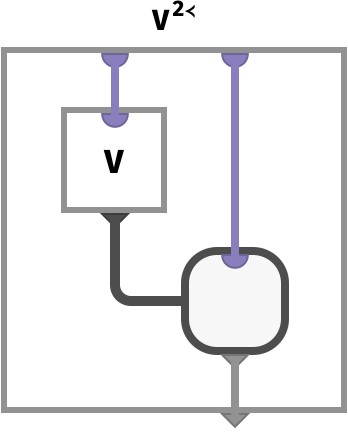
Array circuit #
Here we illustrate the circuit for the nesting of the matrix M to a vector of row-vectors M2≻:
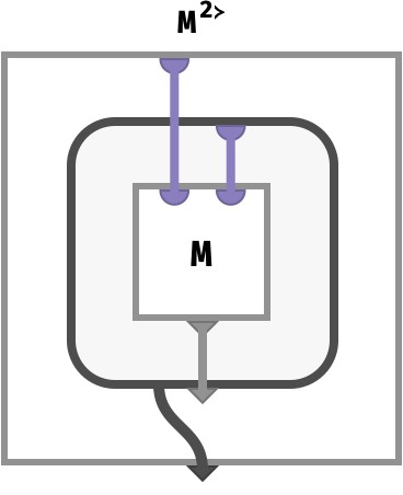
Notice that the value returned here is an entire array, which is defined by the dark gray “bubble”. The type of this array is shown by the pattern of ports on its frame. The frame has one input port (a part) and one output port (a value), and is hence a vector, but its cells are computed by looking up cells in the original matrix M. The thick gray wire indicates that the bubble itself is returned as the output value of our entire array.
Unnest op #
Unnesting is the inverse of nesting. It is only defined on an array of arrays, e.g. an array that is already the result of nesting.
Shapewise, it takes an array of vectors and embeds the vector axis into the array axes at position n:
   A:⟨…⟩ -> ⟨■⟩ -> V
 An≺:⟨…,■n,…⟩ -> V
Here is an example of unnest operating cellwise on a matrix of vectors:
A : ⟨■,■⟩ -> ⟨■⟩ -> V

A1≺[●,●,●] ≡ A[●,●][●]
Needless to say, we have the following general equation:
(An≻)n≺ ≡ A
Array circuit #
Here we depict the circuit for the inverse V2≺ of the row-vector nesting V = M2≻ we illustrated above. It uses the first part of the key to look up the value of a single cell in the vector-of-vectors V. This value is depicted as the gray bubble, which is carried out of V. Since this value is itself a vector, the resulting bubble has an input port and an output port, and this input port is fed using the second part of the key. The resulting value is then returned.
Let’s substitute the circuit we obtained earlier for M2≻ into the diagram above for the box labeled V:
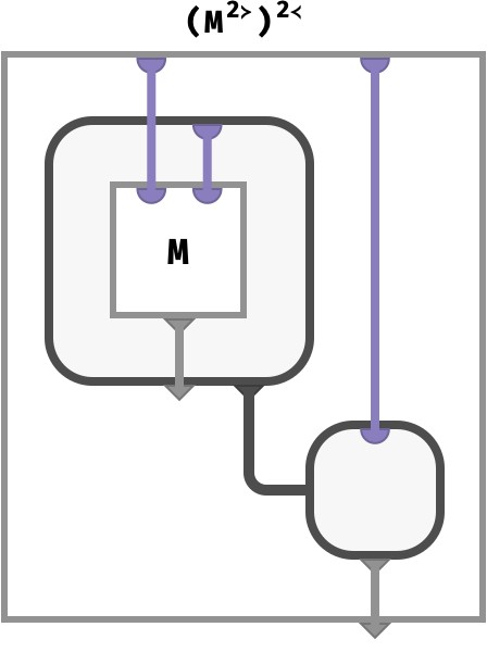
We can now simplify this diagram. The bubble in the top left is where an array value is defined, then the value of this bubble is fed to the bottom right, where it is used. So we can substitute the picture in first blue bubble (the definition of the array), which corresponds to how V = M2≻ is defined, into the second bubble:
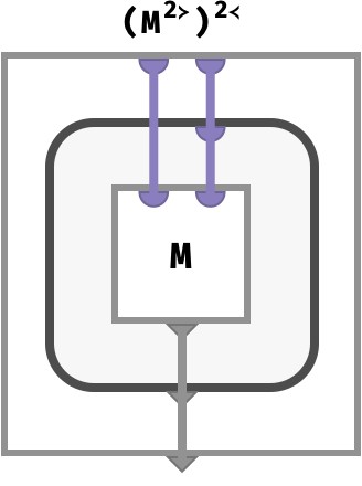
We can now “pop” this single bubble:
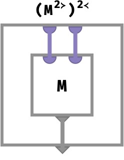
This has been a fun little visual proof that M2≻2≺ = M. Well, I found it fun at least!
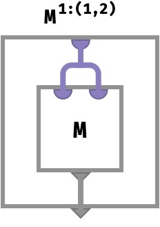
Diagonal op #
Just as broadcasting can be seen as ignoring a part of the key of a derived array, diagonals can be seen as duplicating a part of the key of a derived array. In the first case, the derived array has additional axes; in the second case, the derived array has fewer axes. We write this as An:(m,p) to indicate that the n‘th part of the derived array key is used as the m and p parts of the original array A.
In the simplest case, we can take the diagonal of a square matrix M, which gives us a vector M1:(1,2). Crucially, the part spaces of the duplicated axes must be identical, meaning the matrix M should be square M:⟨N,N⟩. Let’s write the cellwise definition for a matrix diagonal:
    M:⟨N,N⟩ -> V
M1:(1,2):⟨N⟩ -> V

M1:(1,2)[d] ≡ M[d,d]
The corresponding array circuit is:
Let’s work with the following example matrix M:
    ⎡[1 2 3
M = ⎢[4 5 6
    ⎣[7 8 9
The diagonal D = M1:(1,2) has cells:
D[●] ≡ M[●,●]

D[1] ≡ M[1,1] = 1
D[2] ≡ M[2,2] = 5
D[3] ≡ M[3,3] = 9

D = [1 5 9]
Here we can highlight these cells inside the original matrix:
⎡[1 2 3
⎢[4 5 6
⎣[7 8 9
Obviously, this situation can generalize in several ways when we are taking the diagonal of a 3-array, depending on the ways in which we choose to duplicate the key space. Let’s illustrate the possible array circuits for a cubic 3-array A:⟨N,N,N⟩. Note we are coloring the ports and wires of the various arrays to correspond with our axis coloring above. Next to each circuit we where the cells of the diagonal are being taken from A:
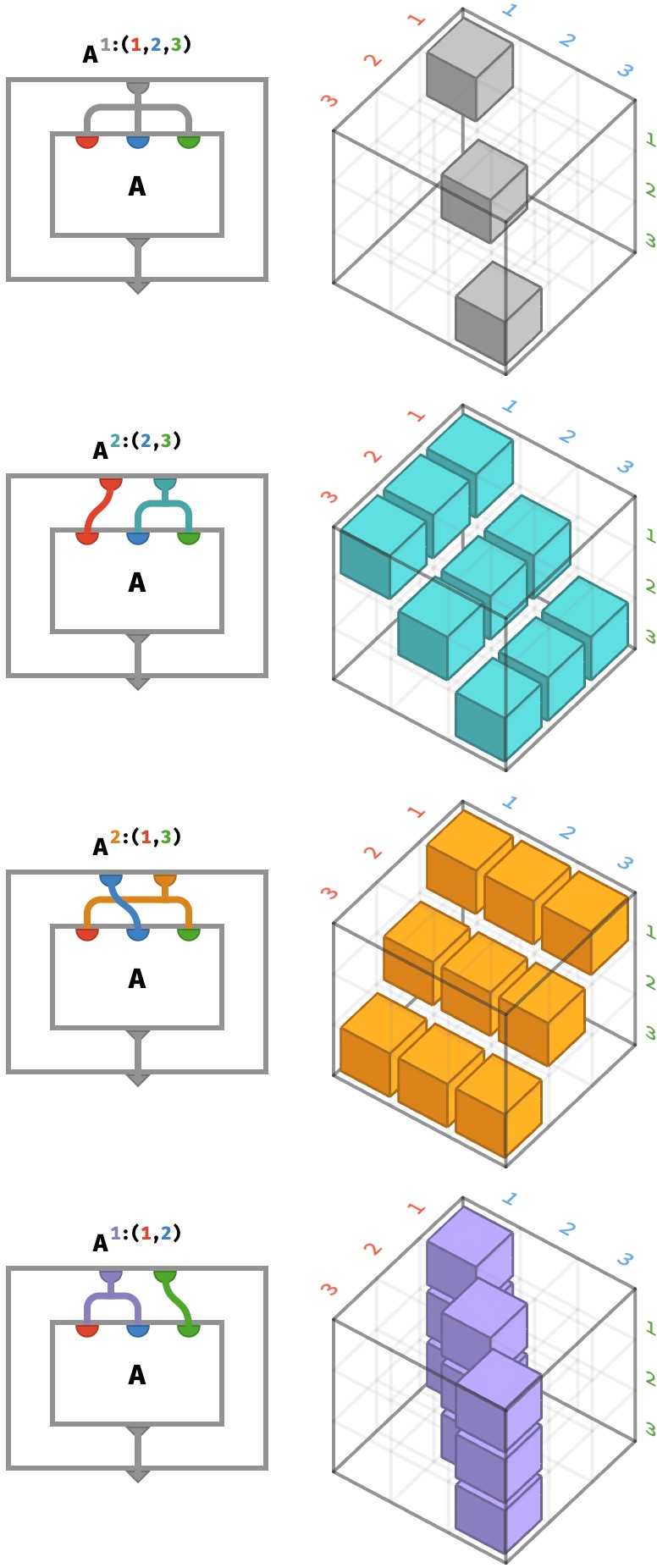
The top circuit depicts the “full diagonal” which yields a vector taken across the cells of a cubic 3-array. The bottom three circuits show three ways of taking the “partial diagonal” to yield a matrix – we also have freedom about where to put the diagonalized axis – which amounts to just transposing the resulting matrix.
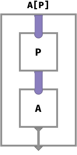
Pick op #
Finally, we can use an array of positions P to pick cells in another array A.
We’ll write this as A[P].
To do this, the value space of the picking array P must be the same as the key space of target array A:
   P : K -> ⟨s1,s2,…⟩
   A :      ⟨s1,s2,…⟩ -> V
A[P] : K                -> V
The cellwise definition is then:
(A[P])[●,●,●,…] = A[P[●,●,●,…]]
But in the functional perspective, this is just the ordinary function composition of “P then A”!
Example 1: picking from a vector A = [10 20 30]:
P = (2)            =>   A[P] = 20
P = [(3) (1) (2)   =>   A[P] = [30 10 20]
P = [[(1)] [(2)]]  =>   A[P] = [[10] [20]]
Example 2: picking from a matrix A = [ [10 20] [30 40] ]:
P = (1,1)                 =>   A[P] = 10
P = [(1,1) (2,2) (2,1)]   =>   A[P] = [10 40 30]
P = [[(2,1)] [(1,2)]]     =>   A[P] = [[30] [20]]
Note we have coloured the parts of the keys in the picking matrix with the colour of the axis of the target array that they correspond to. So, values in P colour code axes in keys of A.
Array circuit #
Here, the picking array P is applied to the input key to obtain a new key that is then looked up in the target array A:
Summary #
This post introduces notation for the theoretical structure of array programming, gives a range of different practical examples to build intuition, and sets the stage for more interesting developments. Next, we’ll discuss rainbow arrays, which make a simple but important change that has major consequences for how we can think about array manipulations.
We’ll end this post with a table of the operations we covered above:
| operation | meaning | cellwise definition |
|---|---|---|
| lift | apply f to matching cells |
f↑(A,B)[…] ≡ f(A[…], B[…]) |
| aggregate | use f to summarize axis |
fn(A)[…] ≡ f●∈■{ A[…,●,…] } |
| merge | collapse parts of an axis together | fRn(A)[…,●,…] ≡ f●∈■{ A[…,●,…] | R(●,●) } |
| broadcast | add constant axis | An➜[…,●,…] ≡ A[…] |
| transpose | permute (reorder) axes | Aσ[…] ≡ A[σ(…)] |
| nest | form array of arrays | An≻[…][●] ≡ A[…,●,…] |
| diagonal | fuse multiple axes together | A1:12[●,…] = A[●,●,…] |
| pick | choose cells by key | A[P][…] ≡ A[P[…]] |
In the next post we will recast these operations in terms of rainbow arrays, in which ordered axes are replaced with coloured axes.